All Chapter Projects

Minding the Hole in the Ozone Layer

As time goes on, there is increasing awareness, controversy, and legislation regarding the ozone layer and other environmental issues. The hole in the ozone layer over the South Pole disappears and reappears in a cyclical manner annually. Suppose that over a particular stretch of time the hole is assumed to be circular with a radius growing at a constant rate of 2.6 kilometers per hour.

Source: NASA

1. Assuming that t is measured in hours, that $t=0$ corresponds to the start of the annual growth of the hole, and that the radius of the hole is initially $0$, write the radius as a function of time, t. Denote this function by $r\left(t\right)$.

2. Use function composition to write the area of the hole as a function of time, t. Denote this function by $A\left(t\right)$. Sketch the graph of $A\left(t\right)$ and label the axes appropriately.

3. After finding $A\left(1\right)$, the area of the ozone hole at the end of the first hour, determine the time necessary for this area to double. How much additional time does it take to reach three times the initial area?

4. Are the two time intervals you found in Question 3 equal? If not, which one is greater? Explain your finding. (Use a comparison of some basic functions discussed in Section 1.2 in your explanation.)

5. What are the radius and area after $3$ hours? After $5.5$ hours?

6. What is the average rate of change of the area from $3$ hours to $5.5$ hours?

7. What is the average rate of change of the area from $5.5$ hours to $8$ hours?

8. Is the average rate of change of the area increasing or decreasing as time passes?

9. What flaws do you see with this model? Can you think of a better approach to modeling the growth of the ozone hole?

Pandemic Predictions

The emergence of the SARS-CoV-2 virus in late 2019 and its subsequent rapid global spread changed the world as we know it. The World Health Organization declared the spread to be a pandemic, known as COVID-19, in March 2020, recommending precautions such as cleanliness, social distancing, and the use of face masks. Mathematics in general, and functions in particular, provide us with the tools to build models that help us understand the spread of contagious diseases and the nature of epidemics or pandemics. This project will provide an introduction to the way such models can be built. Good mathematical models can not only help us understand how an epidemic or pandemic runs its course, but can also be used in decision making regarding mitigation measures and allocation of resources in order to save lives!

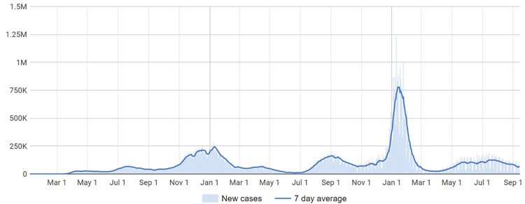
A combination of bar and line graph where the bars represent the number of new cases and the line represents the 7-day average. The x-axis represents months spanning from January 1, 2020 to September 1, 2022. The y-axis represents number of infections spanning from 0 to 1.5 million. The distribution of infections matches the curve of the 7-day average with most of the data staying below 125,000 infections. Between November 1, 2020 and February 1, 2021, the number of infections rises to 250,000 before falling back down. Between December 1, 2022 and March 1, 2022, the number of average infections peaks just over 750,000 while the new cases peaks 1.25 million before falling back down.

Source: Google COVID-19 Open Data (goo.gle/COVID-19-open-data)

COVID-19 was of particular concern early on when there were no vaccines available and the overwhelming majority of the population had not yet been exposed to the virus, making them susceptible to it. In this project, we will build a rudimentary mathematical model to describe and understand the spread of the disease on a college campus of $\mathrm{25,000}$ students, with the following simplifying assumptions.

• Anyone catching the disease eventually recovers.

• After recovery, any affected individual becomes immune (i.e., we will assume there are no reinfections).

• There are no vaccines yet available.

Further, we will partition the campus population into the following three subsets:

• Infected, meaning those students carrying the virus (with or without symptoms)

• Recovered, meaning those students who cannot be reinfected (due to our simplifying assumptions)

• Susceptible, meaning those who have not yet had the virus and can still potentially get it

Note that the sizes of these sets depend on time—that is, they are functions of time—while at any moment in time, they always add up to the total of $\mathrm{25,000}$ students. We will denote these subsets of people by $P_i$, $P_r$, and $P_s$, respectively.

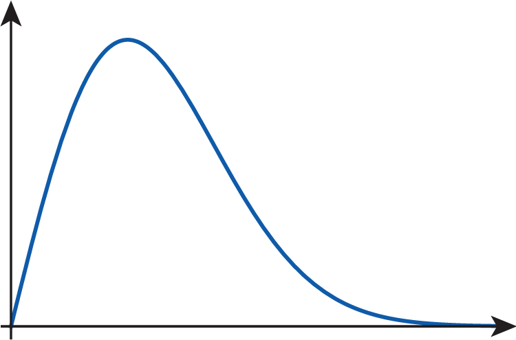
1. Figure 2 illustrates how the size of the infected subpopulation $P_i$ may depend on time t.

   

   The first quadrant of a cartesian graph with an unlabeled curve. The curve starts at the origin and rises quickly and begins descending similarly but the descent slows as it continues.

   1. What are the independent and dependent variables of this function?

   2. Use the features of the graph to explain why it seems realistic. What does it tell you about the way the infection runs its course on campus?

   3. Use function notation to write an equation expressing the fact that the numbers of infected, recovered, and susceptible student populations sum up to $\mathrm{25,000}$ at any given time. (Hint: remember that $P_i$, $P_r$, and $P_s$ are functions of time t.)

2. How would you expect the number of susceptible students to change over time? Explain and sketch a possible graph of the size of $P_s$ over time.

3. Answer Question 2 and sketch a possible graph for the recovered subpopulation $P_r$.

Throughout the COVID-19 pandemic, the daily reports included (among other data) the number of new cases on a given day. Note that this is an important measure of how fast the infection spreads. In other words, using the general concept of "rate" being "change divided by time," you can think of that number as the rate of increase in size of the set of people who have caught the disease. (You will learn more about rates starting in Chapter 2.) Throughout the next few questions, we are going to build an equation modeling the progression of the disease in the college population. Our assumptions will be as follows. New infections are always the result of interactions between members of the infected and susceptible populations. Even though not all interactions result in new infections, a certain percentage of them do (note that this percentage can be decreased by mitigation measures, such as masking or distancing). We will assume that the number of interactions is directly proportional to both $P_s$ and $P_i$.

4. Find a formula for $N\left(t\right)$, the number of daily new infections, given the assumptions above. (The constant of proportionality in this case is called the transmission coefficient. Let us denote it by b.)

5. Given that, on average, an infected person is contagious for about ten days, explain why we can expect approximately ${\displaystyle \frac{P_i\left(t\right)}{10}}$ students to recover daily. Discuss the limitations of this model.

6. 1. Given that some students get infected while others recover every single day, use your answers to Questions 4 and 5 to find a formula for $\widehat{P_i}\left(t\right)$, the daily increase in numbers of the infected student population.

   2. Use your formula to predict the number of new infections on a day when $500$ students are carrying the virus and $1000$ have already recovered. Use the value $b=0.000025$ for the transmission coefficient.

7. Use the equation obtained in Question 6 to predict the size of the susceptible population (i.e., those who have not caught the virus) when the epidemic peaks on campus. (Hint: Find what value of $P_s$ predicts a zero daily increase in $P_i$ for the first time. Round to the nearest integer. Then check that the following day, the predicted daily increase in $P_i$ is negative.)

Before Unlimited Calls

Some years ago, it was common for long-distance phone companies to charge their customers in one-minute increments. In other words, the company charges a flat fee for the first minute of a call and another fee for each additional minute or any fraction thereof (see Exercise 82 in Section 2.5). In this project, we will explore in detail a function that gives the cost of a telephone call under the above conditions.

1. Suppose a long-distance call costs $75$ cents for the first minute plus $50$ cents for each additional minute or any fraction thereof. In a coordinate system where the horizontal axis represents time t and the vertical axis price p, draw the graph of the function $p=C\left(t\right)$ that gives the cost (in dollars) of a telephone call lasting t minutes, $0<t\le 5$.

2. Does $\underset{t\to \mathrm{1.5}}{\lim }C\left(t\right)$ exist? If so, find its value.

3. Does $\underset{t\to 3}{\lim }C\left(t\right)$ exist? Explain.

4. Write a short paragraph on the continuity of this function. Classify all discontinuities; mention one-sided limits and left or right continuity where applicable.

5. In layman's terms, interpret $\underset{t\to \mathrm{2.5}}{\lim }C\left(t\right)$.

6. In layman's terms, interpret $\underset{t\to 3^{-}}{\lim }C\left(t\right)$.

7. In layman's terms, interpret $\underset{t\to 3^{+}}{\lim }C\left(t\right)$.

8. If possible, find $C^{\prime }\left(3.5\right)$.

9. If possible, find $C^{\prime }\left(4\right)$.

10. Find and graph another real‑life function whose behavior is similar to that of $C\left(t\right)$. Label the axes appropriately and provide a brief description of your function.

The Squirrel Population Is Going Nuts

When there is an ample food supply, ideal conditions, and no limiting factors that would curb birth rates or cause premature death, a population is expected to grow quickly and at an accelerating rate. An easy way to understand this is to consider the fact that as the population grows, there will be more and more births and, at least initially, deaths won't affect the growth very much. If we examine a population over a longer time span, however, we would expect the growth rate to slow down. This may be due to limitations in food supply, the appearance of predators, diseases, or other factors. (You will learn more about population growth in Section 3.7.)

In this project, we will examine a few patterns of population growth, discuss rates, and look at some functions that can be used to describe the process.

1. 1. Suppose a population of one hundred squirrels starts to grow in a large forest with unlimited food supply and no predators. Using the horizontal axis to represent time t in months and the vertical axis to represent the number of squirrels in the population, sketch by hand a possible graph depicting the population growth during the first few months. Explain your choice, mentioning rate of change, and how it changes over time. (Answers will vary.)

   2. Use a graphing utility to find and display the graph of a function that approximates your sketch from part a. reasonably well. What type of function did you use and why? (Hint: Pay attention to the scaling of the axes. You may want to review the common functions and function transformations from Sections 1.2 and 1.3. Answers will vary.)

2. 1. Now assume that the growth of the population in Question 1 starts slowing significantly after the first year. Sketch by hand a possible graph of the population growth over the first two years. Compare and contrast this new graph with the graph you sketched in Question 1a and explain any similarities and differences.

   2. * Like you did above in Question 1b, utilize a graphing utility to find a formula for a function that closely approximates your sketch for Question 2a.

3. Write a short paragraph to argue why it is unrealistic to model the growth of a population using a curve that is increasing at an increasing rate on $\left(0,\mathrm{\infty }\right)$. Describe the kind of graph that you think would be the better choice.

4. 1. Hand sketch a possible curve depicting the growth of a squirrel population that has grown large enough to reach the limit of the amount of food that the environment is able to supply. How does the rate of change vary over time? Explain your reasoning.

   2. How do you think the curve might change if it is to reflect the appearance of a growing predator population?

The first mathematician to introduce accurate models for population growth was Pierre François Verhulst (1804–1849). He introduced what he called logistic curves in a series of papers starting with "Note on the law of population growth," published in 1838. His work was based on studying the population growth patterns of several countries, including his native Belgium. In Question 5, you will be asked to examine such a logistic curve.

5. The function below describes the growth of a squirrel population in a large, forested area; time is measured in months, the number of squirrels in thousands.

   $P\left(t\right)={\displaystyle \frac{90}{1+74e^{-5\mathrm{t}}}}$

   1. Determine the limit of the function as $t\to \infty$. Describe in words the real-life meaning of the answer.

   2. Use a graphing utility to sketch the graph of $P\left(t\right)$. How does its derivative change with time (i.e., as $t\to \infty$)?

6. The following table represents the approximate size of the US population between the years 1940 and 2020. Use the table to answer the questions below.

   Approximate Size of the US Population in Millions

   Year	1940	1950	1960	1970	1980	1990	2000	2010	2020
   Population (in millions)	$132.2$	$151.3$	$179.3$	$203.2$	$226.5$	$248.7$	$281.4$	$308.7$	$331.4$

   1. Find the average annual rate of change of the population of the US between 1950 and 2000.

   2. Estimate the annual rate of change of the US population in the year 1950. (Hint: Consider the population before and after 1950.)

   3. Estimate the annual rate of change of the US population in the year 2000. (See the hint given in part b.)

   4. Compare the answers you obtained in parts a.–c. What can you infer from this? How does the rate seem to change over time?

   5. Using the population data from the table, hand sketch a possible graph depicting the population change between 1940 and 2020. How is your answer to part d. reflected in the graph?

   6. Based on your answers above, what are your predictions for the short-term and long-term future?

Under Pressure

The following table shows the atmospheric pressure p at the altitude of k feet above sea level (pressure is measured in mm Hg; note that this unit of pressure is approximately the pressure generated by a column of mercury $1$ millimeter high).

1. Find the average rate of change of air pressure from sea level to $2000$ feet of altitude.

2. Find the average rate of change of air pressure between the altitudes of $4000$ and $\mathrm{10,000}$ feet.

3. Use a symmetric difference quotient

   ${\displaystyle \frac{p\left(c+h\right)-p\left(c-h\right)}{2h}}$

   to estimate the instantaneous rate of change of air pressure at $7000\mathrm{ft}$ by choosing $h=1000\mathrm{ft}$.

4. Tell whether you expect the answer to Question 2 or 3 to better approximate the instantaneous rate of change of air pressure at altitude $7000\mathrm{ft}$. Explain. (Hint: Plotting the data on paper may help.)

5. * Explain why you expect the symmetric difference quotient ${\displaystyle \frac{f\left(c+h\right)-f\left(c-h\right)}{2h}}$ in general to be a better approximation of the instantaneous rate of change of f at $x=c$ than the "regular" difference quotient ${\displaystyle \frac{f\left(c+h\right)-f\left(c\right)}{h}}$.

6. Use a graphing utility to find an exponential regression curve to the given data and plot the curve along with the data on the same screen.

7. Use the exponential function you found in Question 6 to estimate the instantaneous rate of change of air pressure at $7000\mathrm{ft}$, and compare with your estimate given in Question 3.

8. Is the instantaneous rate of change increasing or decreasing with altitude? Explain.

The Ultimate Hail Mary

In April 2021, legendary NFL tight end Rob "Gronk" Gronkowski set a world record by catching a football that was dropped from a helicopter hovering $600\mathrm{ft}$ overhead. In the words of ESPN's Adam Schefter, this was the "highest altitude catch" ever! In this project, we will examine the behavior of objects dropped from high altitudes. Throughout Questions 1–5, we will ignore air resistance; then in Questions 6–8, we will develop the tools to include it in our calculations, allowing us to make our predictions much more accurate.

1. An object is dropped from the window of a hovering helicopter at an altitude of $250\mathrm{ft}$. How long is it in the air and what is its speed of impact?

2. Answer Question 1 under the assumption that the object is dropped from the same altitude from a helicopter that is ascending vertically with a constant speed of $16{\displaystyle \frac{\mathrm{ft}}{\mathrm{s}}}$.

3. What happens if the helicopter is accelerating vertically upward at $0.5{\displaystyle \frac{\mathrm{ft}}{{\mathrm{s}}^2}}$ but its altitude and instantaneous upward velocity are the same as in Question 2 at the moment the object is dropped? Explain.

4. Based on your answers given above, do you think the situation for Gronk would have been different if the football had been dropped from a vertically ascending or descending (rather than hovering) helicopter? Explain.

5. Answer Question 1 if an object is dropped from a helicopter hovering at an altitude of $600\mathrm{ft}$. Is your answer realistic? Could this have been true of the football Gronk caught? Explain.

In order to develop a model to more accurately reflect (and predict) what happens in real-life free falls, we must consider air resistance. From your answers to the next questions, you will be able to better approximate the actual speed of the football when Gronk caught it. It was indeed a highly impressive feat!

6. When air resistance is taken into account, does a free-falling object constantly accelerate throughout its motion? If not, what can you say about its acceleration and velocity? Explain. (Hint: Think of falling rain drops or snowflakes.)

7. The resistance of the medium surrounding a moving object exerts a force directly opposing the motion. That force, commonly called the drag force, is obtained from the formula

   $F_d={\displaystyle \frac{1}{2}\rho v^2{C}_{d}A}$

   where v is the velocity and A is the cross-sectional area of the moving object, ρ stands for the density of the surrounding medium, and $C_d$ is called the drag coefficient, which depends on the general shape of the object. (Note that A is actually the area of the cross-section perpendicular to the direction of motion. Can you see why?)

   Use Newton's Second Law of Motion (see Topic 2 in Section 3.7) to find a formula for the maximum velocity that a free-falling object attains when falling in air. This is called the object's terminal velocity. (Assume that the altitude is not high enough to affect air density.)

8. 1. Use your answer to the previous question to estimate the speed of the falling football at the moment Gronk caught it, setting a world record. (Hint: We will assume that the ball was falling with its major axis oriented horizontally and approximate its cross-section as an ellipse. The formula for the area of an ellipse can be found in Example 3 of Section 7.4.) A football's major and minor axes are $11$ and $7\mathrm{in.}$, respectively, and its mass is approximately $0.9\mathrm{lb}$. Use $0.77$ for the drag coefficient of a football falling with its major axis perpendicular to the direction of the fall. Use $0.075{\displaystyle \frac{\mathrm{lb}}{{\mathrm{ft}}^3}}$ for air density.

   2. Compare the above result to your answer given in Question 5. How significant is the effect of air resistance on a falling football? Do you think the same would be true of a falling rock? Why?

   3. Considering your answers above, how do you think you need to modify your answers to Questions 1–4 when air resistance is taken into consideration? Explain.

Spot the Difference

Consider a function $f\left(x\right)$ that is at least twice differentiable. In this project, you will show that the second derivative of $f\left(x\right)$ at $x=c$ can be found as the limit of so-called second-order differences, as follows.

$f^{″}\left(c\right)=\underset{h\to 0}{\lim }{\displaystyle \frac{f\left(c+h\right)-2f\left(c\right)+f\left(c-h\right)}{h^2}}$

1. Instead of working with a secant line through the points $\left(c,f\left(c\right)\right)$ and $\left(c+h,f\left(c+h\right)\right)$ like we did when approximating the first derivative, suppose that

   $y=a_1{x}^2+a_{2}x+a_3$

   is the parabola through the following three points on the graph of f: $\left(c-h,f\left(c-h\right)\right)$, $\left(c,f\left(c\right)\right)$ and $\left(c+h,f\left(c+h\right)\right)$. Do you expect to always be able to find coefficients $a_1,a_2,a_3\in ℝ$ such that the resulting parabola satisfies the desired conditions? Why or why not? Why would you expect $2a_1$ to be "close” to $f^{″}\left(c\right)$ if h is "small”? What will happen to $2a_1$ as $h\to 0$? Write a short paragraph answering the above questions.

2. By substituting the points $\left(c-h,f\left(c-h\right)\right)$, $\left(c,f\left(c\right)\right)$, and $\left(c+h,f\left(c+h\right)\right)$ into $y=a_1{x}^2+a_{2}x+a_3$, obtain a system of linear equations in unknowns $a_1$, $a_2$, and $a_3$. Solve the system for the unknown $a_1$.

3. Use Questions 1 and 2 to argue that $f^{″}\left(c\right)$ is the following limit of the second‑order differences.

   $f^{″}\left(c\right)=\underset{h\to 0}{\lim }{\displaystyle \frac{f\left(c+h\right)-2f\left(c\right)+f\left(c-h\right)}{h^2}}$

4. Use L'Hôpital's Rule to verify the result you found in Question 3.

Cutting Corners with Cappuccinos

Suppose the management of a coffee shop chain wants to minimize the daily costs associated with delivery and storage for its franchises. In this project, we will find a formula for accomplishing that, given certain simplifying assumptions.

We will assume that the holding costs for a franchise are directly proportional to storage time as well as the total amount of unsold (whole bean or ground) coffee they have on hand. (Holding costs in general are the costs associated with storing unsold inventory. Some of the contributors to these expenses are the facts that the capital already invested in the inventory cannot earn interest elsewhere, as well as the costs of storage space, utilities, insurance, labor, damaged or spoiled items, etc.) We will assume that each delivery comes with a flat charge, regardless of the amount of coffee delivered. In addition, daily consumer demand is assumed to be constant, meaning the total amount of coffee purchased at the franchise is a linear function of time. Our notation will be the following.

1. Suppose a delivery in the amount of $a_0$ pounds of coffee arrives at a franchise. In a coordinate system where the horizontal axis represents time t measured in days and the vertical axis stands for the amount A of coffee measured in pounds, sketch the graph of $A\left(t\right)$, the amount of coffee at the store as a function of time, from the point of delivery until the store runs out of supplies. What type of function is it? (Suppose delivery happens at $t=0$. Be careful. Neither time, nor the coffee amount stored, can ever be negative.)

2. Using $a_0$ and c as parameters (unspecified, but fixed values), answer the following questions.

   1. Find the equation of the graph you sketched in Question 1.

   2. Use your answer from part a. to find a formula for $t_0$, the number of days it takes for the franchise to run out of supplies. This length of time is called days sales of inventory, or DSI in the business world.

3. Suppose that during the first day after delivery, the franchise's coffee supply decreases from the initial $a_0$ pounds to $a_1$ pounds. Explain why it is reasonable to calculate their holding cost for the day as follows.

   $H_1={\displaystyle \frac{a_0+a_1}{2}h}$

   (In other words, by multiplying the average daily inventory by the holding cost per pound per day. Hint: Refer to Question 1.)

4. Now consider the first two days of the DSI cycle. Assuming that there are still $a_2$ pounds of coffee left at the end of the second day, use your answer to Question 3 to show that the total holding costs the franchise incurs during the first two days of the cycle can be obtained as follows.

   $H_2={\displaystyle \frac{a_0+a_2}{2}\left(2h\right)}=\left(a_0+a_2\right)h$

   (In other words, we can again take the average inventory for the first two days and multiply by twice the daily holding cost per pound of coffee.)

5. Generalizing the result from Question 4, answer the following questions.

   1. Find a formula for the total holding cost $H_{t_0}$ for a full DSI cycle of $t_0$ days. (Hint: Use the fact that the amount stored at the endpoint of the cycle is zero pounds, and again work with the average inventory.)

   2. Find a formula for the total cost $C_{t_0}$ incurred by the franchise from delivery and storage over the cycle in part a.

The remainder of this project is devoted to finding a formula for the length of the DSI cycle that minimizes the storage-anddelivery expenses for a franchise. Customer demand, the delivery fee, and the daily holding costs per pound will be assumed to be constant, but we will treat the delivery amount and the length of the DSI cycle as variables (denoted by a and x, respectively). As you might have discovered already from answering Questions 1–4, the delivery amount will determine the length of time before the next shipment becomes necessary; in other words, the two variables are strongly related.

6. Letting a denote the amount of coffee (in pounds) delivered to the franchise and x stand for the time it takes (in days) for the store to run out of supplies, answer the following.

   1. Find an equation relating the variables a and x. (Hint: Refer to Question 2b.)

   2. Use your answers from Questions 5b and 6a to express the total cost C as a function of DSI cycle length; that is, find a formula for the function below.

      $C=C\left(x\right)$

   3. Find a formula for the function $D\left(x\right)$, the average daily cost stemming from delivery and storage expenses. (Hint: There are x days in a DSI cycle.)

7. Find the (positive) critical point of the daily cost function $D\left(x\right)$ of Question 6c, and use the Second Derivative Test to obtain a formula for the length of the DSI cycle that minimizes the daily delivery and storage-related expenses for the franchise.

8. Sketch a possible graph for the daily cost function $D\left(x\right)$. Briefly discuss the main features of the graph.

Looking For a Sine

The topic of this project is the so-called sine integral function, which is important for its applications, most notably in electrical engineering and signal processing.

1. Consider the following piecewise‑defined function.

   $f\left(t\right)=\{\begin{array}{ll}{\displaystyle \frac{\sin t}{t}}& \text{if }t>0\hfill \\ 1& \text{if }t=0\hfill \end{array}$

   Prove that for any $x\ge 0$, $f\left(t\right)$ is integrable on $\left[0,x\right]$.

2. The sine integral function is defined as follows.

   $\mathrm{Si}\left(x\right)={\displaystyle {\int }_0^{x}f\left(t\right)\mathit{d}t}$, for $x\ge 0$

   Prove that $\mathrm{Si}\left(x\right)$ is continuous.

3. Find the derivative ${\displaystyle \frac{\mathit{d}}{\mathit{d}x}}\mathrm{Si}\left(x\right)$.

4. Without graphing first, write a short paragraph on why you would expect the graph of $\mathrm{Si}\left(x\right)$ to be oscillating. Explain why its amplitude is expected to decrease as $x\to \infty$.

5. Find the x‑values where the relative maxima and minima of $\mathrm{Si}\left(x\right)$ occur.

6. Extend the definition of $\mathrm{Si}\left(x\right)$ to negative x‑values and prove that for any $a>0$, ${\displaystyle {\int }_{-a}^a\mathrm{Si}\left(x\right)\mathit{d}x}=0$.

7. Use a graphing utility to plot the graph of $\mathrm{Si}\left(x\right)$ on the interval $\left[-8\pi ,8\pi \right]$.

8. Use a graphing utility to approximate the range of $y=\mathrm{Si}\left(x\right)$ to four decimal places.

Too Math Too Furious

When we talk about acceleration of cars (for example, when discussing times necessary to accelerate from zero to sixty miles per hour), we often assume their acceleration is constant. This makes it easy to perform speed and distance calculations (see Question 1 below). However, in real life, constant acceleration over long periods of time may not be realistic. Air resistance, an engine's torque delivery, changing road conditions, and potential wheel spin can all lead to variable acceleration. Air drag alone, which is proportional to the square of velocity, has a strong effect on acceleration (see Question 7 of the Chapter 3 Application Project). For example, at the very high speeds experienced by race cars, air resistance is strong enough that simply stepping off the accelerator creates a sense of hitting the brakes with full force! It would therefore be realistic to expect acceleration to decrease at higher speeds. In this project, we will illustrate the power of integration by considering motion problems where the accelerating vehicles have time-dependent (nonconstant) acceleration. We will start with an ultrafast Porsche model.

1. The 2021 Porsche 911 Turbo S reaches $150\mathrm{mph}$ from a standstill in $13.6$ seconds. In the analysis that follows, we will initially use the (unrealistic) simplifying assumption that acceleration is constant throughout the $0$–$150\mathrm{mph}$ test run.

   1. Find the presumably constant acceleration a (in ${\displaystyle \frac{\mathrm{ft}}{{\mathrm{s}}^2}}$).

   2. Use antidifferentiation (as in Example 4 of Section 4.7) to find the accelerating car's velocity $v=v\left(t\right)$ as a function of time (in ${\displaystyle \frac{\mathrm{ft}}{\mathrm{s}}}$).

   3. Find an integral formula for the velocity function in part b. (Hint: Use the Fundamental Theorem of Calculus, Part I.)

   4. Find the distance (in feet) covered by the car during the acceleration run.

2. The table below shows the actual acceleration times of the 2021 Porsche 911 Turbo S from zero to various speeds up to table below shows the actual $150\mathrm{mph}$. (Units are in miles per hour and seconds. As a side note, the car is actually capable of a top speed of table below shows the actual $205\mathrm{mph}$!)

   2021 Porsche 911 Turbo S Acceleration Times

   Increase in Speed ($\mathrm{mph}$)	$0$–$30$	$0$–$40$	$0$–$50$	$0$–$60$	$0$–$70$	$0$–$80$	$0$–$90$	$0$–$100$	$0$–$150$
   Time ($\mathrm{s}$)	$0.9$	$1.4$	$1.8$	$2.3$	$3.0$	$3.7$	$4.5$	$5.6$	$13.6$
   Source: Motor Trend

   1. Use the data from Table 1 to explain why the acceleration $a=a\left(t\right)$ is actually a nonconstant function of time, rendering our simplifying assumption in Question 1 unrealistic.

   2. What features would you anticipate for the graph of $a\left(t\right)$ to possess? Describe these features, mentioning the first derivative and concavity. (You may want to plot a few points using data from the table.)

Notice that Table 1 gives us values of the Porsche's velocity function $v=v\left(t\right)$ at various points on the time axis during the acceleration run. We will use these values to approximate the total distance covered during the run. (Note that this is the same as the displacement of the car from its starting position, since there is no change of direction during this type of test run.) To start off, notice from Table 1 that the Porsche reaches $30\mathrm{mph}$ in the first $0.9$ seconds. A crude approximation of the distance covered while doing so can be obtained by taking the average of the speeds at the two endpoints of this time interval, at $t=0$ and $t=0.9$ (where the speeds are $0\mathrm{mph}$ and $30\mathrm{mph}$, respectively), and assuming that the speed is constant and equal to this average value throughout the entire time interval.

3. 1. Use the technique described above to approximate the displacement during the first $0.9$ seconds of the run, and then on the second time interval, from $0.9$ seconds to $1.4$ seconds. Add up the results to obtain an estimate for the total displacement during the first $1.4$ seconds of the run. Express your answer in feet.

   2. Continue the process from part a. over all consecutive time intervals from Table 1 and add up the results to obtain an estimate for the total displacement (in feet) during the entire $0$–$150\mathrm{mph}$ acceleration run. What is the name of the sum you just formed?

Notice that if we had more data in Table 1, we could work with shorter time intervals in order to arrive at more accurate estimates for displacement. Better yet, if we had a formula for $v=v\left(t\right)$, we could use a definite integral to calculate the actual displacement, much like we did in Example 1 of Section 5.2. You can use this observation to answer Question 4. Then, in the subsequent problems, we will generalize our analysis.

4. Use your work on Question 3 to give a definite integral interpretation of the total distance d traveled by the Porsche during its acceleration run. Find a formula in terms of $v\left(t\right)$.

5. Suppose an object is accelerating along a straight line from $t=t_0$ to $t=t_1$ and its acceleration is given by $a=a\left(t\right)$, while its velocity is $v=v\left(t\right)$.

   1. Use the definite integral to give a formula for the total displacement of the object in terms of $v\left(t\right)$. (Hint: Generalize your answer to Question 4.)

   2. Given $v\left(t\right)$, find an integral formula for the displacement function $d\left(t\right)$ on the interval $\left[t_0,t_1\right]$. (Hint: Generalize your answer to part a.)

   3. Use $a\left(t\right)$ and integration to arrive at an integral formula for the velocity function $v\left(t\right)$ on the interval $\left[t_0,t_1\right]$ (Hint: Generalize your answer to Question 1c.)

   4. Explain the validity of the formula you have given in part c. above. Use Riemann sums in your argument.

6. An experimental race car starts at a standstill and accelerates in a straight line. Suppose its acceleration can be described by the function $a\left(t\right)=\left(31-2t\right){\displaystyle \frac{\mathrm{ft}}{{\mathrm{s}}^2}}$.

   1. What is its velocity (in $\mathrm{mph}$) five seconds later?

   2. How far is it from the start at that instant?

   3. Use technology to find the vehicle's quarter‑mile time. (This means the time needed for it to run a quarter mile from its starting point.)

A Frictionless Flight

In this project, we will expand upon our explorations from Exercises 48 through 55 of Section 6.5 (also see the discussion preceding those exercises). In particular, we will determine an equation satisfied by the velocity of a projectile launched with initial velocity $v_0$, taking into consideration that acceleration caused by gravity decreases with altitude. (This is important when objects are launched to great altitudes.) We will then use our equation to find the maximum height attained by the projectile. This will lead us to the value of the so-called escape velocity, the velocity needed for an object to be able to overcome Earth's gravitational field without further propulsion. (In turn, since gravity is conservative, this is the same velocity an object would achieve if pulled in by gravity from an "infinite distance.") We are ignoring all retarding forces (such as air resistance or friction) in this discussion.

1. Recall from Exercise 48 of Section 6.5 that g, the acceleration caused by gravity on a free‑falling mass near Earth's surface, is approximately

   $g={\displaystyle \frac{MG}{R^2}}$,

   where M and R are the mass and radius of Earth, respectively, and G is the universal gravitational constant. However, a launched projectile's acceleration caused by gravity is negative (if we are assuming the positive direction is upward) and actually depends on its height h above Earth's surface. In particular, use Newton's Law of Gravitation to show that this dependence is given by the equation

   $a\left(h\right)={\displaystyle \frac{-g{R}^2}{{\left(R+h\right)}^2}}$,

   where $a\left(0\right)=-g$, as we would expect. (Actually, $a\left(h\right)\approx -g$ when h is negligible compared to Earth's radius.)

2. Show that if $v=v\left(h\right)$ denotes the velocity of the projectile, then

   ${\displaystyle \frac{\mathit{d}}{\mathit{d}h}}\left(v^2\right)=2{\displaystyle \frac{\mathit{d}v}{\mathit{d}t}}$.

   (Hint: Use the Chain Rule.)

3. Use the above results to show that

   ${\displaystyle \frac{\mathit{d}\left(v^2\right)}{\mathit{d}h}}={\displaystyle \frac{-2g{R}^2}{{\left(R+h\right)}^2}}$.

4. Integrating both sides of the preceding equation with respect to h, show that $v=v\left(h\right)$ satisfies the equation

   $v^2=v_0^2-2gR\left(1-{\displaystyle \frac{R}{R+h}}\right)$.

   (Hint: After integrating, use the fact that $v\left(0\right)=v_0$.)

5. Use the equation found in Question 4 to find the maximum height attained by the projectile. (Hint: Use the fact that $v=0$ when the projectile reaches its maximum height.)

6. Find a formula for the escape velocity $v_e$ of the projectile; then use the data found in the exercises of Section 6.5 (Exercises 48-55 and the preceding discussion) to express your answer in kilometers per second. (Hint: Use the fact that if $v_0=v_e$, the projectile will "travel to infinity.")

7. Find the escape velocity of the projectile if it is launched on the moon. (Hint: For moon data, see Exercise 53 of Section 6.5.)

3 Calculations to Blast Off!

In this project, we will examine the motion of a rocket after launch. As you know, a rocket is propelled by the force caused by the exiting hot gases that result from rapidly burning fuel. This force is called the thrust of the rocket. The difficulty of analyzing rocket propulsion arises from the fact that the mass of the fuel, which comprises a large portion of the rocket's mass, decreases rapidly during flight due to the high rate of fuel burn. This rapid decrease in mass occurs up until the moment when all fuel is used up (a moment known as the burnout point). This means that the net force acting on the rocket is also a nonconstant function of time but, as you will discover, integration helps us overcome the challenge of rapidly changing mass. Throughout the project, we will ignore air resistance and assume that the acceleration caused by gravity $g\approx 9.81{\displaystyle \frac{\mathrm{m}}{{\mathrm{s}}^2}}$ is constant (in the case of rockets that fly to high altitudes, this is not necessarily the case).

Under the above assumptions, we use Newton's Second Law of Motion to obtain the following equation:

$F_n\left(t\right)=F_t\left(t\right)-m\left(t\right)g=m\left(t\right)a\left(t\right)$,  (1)

where $F_t$ denotes the propelling force or thrust. This force arises from the fact that the mass of the burnt fuel is rapidly leaving the rocket-fuel system, thus giving it upward momentum.

Although we omit the details of deriving it here, we will also use the fact that the thrust can be obtained as the product of $v_f$, the relative speed at which the burnt fuel is exiting the rocket, and the rate of decrease in mass:

$F_t\left(t\right)=v_f\cdot {\displaystyle \frac{\mathit{d}m\left(t\right)}{\mathit{d}t}}$.

1. Suppose a rocket of mass eighteen metric tons is fired vertically upward. Of its total mass, fuel accounts for twelve metric tons. The hot gases resulting from burned fuel are leaving the rocket at a relative speed of $2500$ meters per second and at a rate of $150$ kilograms per second. Calculate the thrust $F_t$ propelling the rocket upward.

2. Use Equation (1) to calculate the net force $F_n$ acting on the rocket

   1. at the moment of blastoff;

   2. just before all fuel burns away;

   3. after all fuel has burnt away.

3. Use Equation (1) to find the rocket's velocity function $v\left(t\right)$, as follows. From Equation (1), we obtain

   $m\left(t\right)a\left(t\right)=m\left(t\right)\cdot {\displaystyle \frac{\mathit{d}v\left(t\right)}{\mathit{d}t}}=v_f\cdot {\displaystyle \frac{\mathit{d}m\left(t\right)}{\mathit{d}t}}-m\left(t\right)g$;

   then we use differential notation to arrive at

   $m\mathit{d}v=v_f\mathit{d}m-mg\mathit{d}t$.

   Use this equation to solve for $\mathit{d}v$, and then obtain $v\left(t\right)$ by integration:

   $v\left(t\right)={\displaystyle {\int }_0^t\mathit{d}v}$.

4. Use your answer to Question 3 to find the terminal velocity of the rocket after all fuel has been used up. (Hint: Be careful. The velocity of the exiting fuel is negative.)

Infinite Wisdom

In this project, we will derive a famous infinite product named after its discoverer, the English mathematician John Wallis (1616–1703). Wallis introduced the symbol $\mathrm{\infty }$ for infinity, and in turn he used ${\displaystyle \frac{1}{\infty }}$ to denote an infinitesimal quantity. He contributed to the development of infinitesimal calculus (it wasn't until the 19^th century that infinitesimals were replaced by limits in the works of Bolzano, Cauchy, and Weierstrass).

1. For a nonnegative integer n, let

   $I_n={\displaystyle {\int }_0^{{\displaystyle \frac{\pi }{2}}}{\sin }^{n}x\mathit{d}x}={\displaystyle {\int }_0^{{\displaystyle \frac{\pi }{2}}}{\cos }^{n}x\mathit{d}x}$.

   Find $I_0$, $I_1$, $I_2$, and $I_3$.

2. Show that if $n\ge 2$,

   $I_n={\displaystyle \frac{n-1}{n}}{I}_{n-2}$.

   (Hint: See Exercise 81 of Section 7.1.)

3. Use Questions 1 and 2 to find $I_4$, $I_5$, $I_6$, and $I_7$.

4. Show that in general,

   $I_{2n}={\displaystyle \frac{2n-1}{2n}\cdot \frac{2n-3}{2n-2}\cdot \frac{2n-5}{2n-4}\cdot \dots \cdot \frac{1}{2}\cdot \frac{\pi }{2}}$,

   while

   $I_{2n+1}={\displaystyle \frac{2n}{2n+1}\cdot \frac{2n-2}{2n-1}\cdot \frac{2n-4}{2n-3}\cdot \dots \cdot \frac{2}{3}}$.

   (Hint: Observe a pattern or use induction.)

5. Use Question 4 to show that

   ${\displaystyle \frac{I_{2n}}{I_{2n+1}}={\displaystyle \frac{3^2{5}^2\cdot \dots \cdot {\left(2n-1\right)}^2\left(2n+1\right)}{2^2{4}^2\cdot \dots \cdot {\left(2n\right)}^2}}\cdot {\displaystyle \frac{\pi }{2}}}$

   holds for all n.

6. Show that

   ${\displaystyle \frac{I_{2n-1}}{I_{2n+1}}=1+\frac{1}{2n}}$.

7. Prove the inequalities

   $I_{2n-1}\ge I_{2n}\ge I_{2n+1}$.

   (Hint: Use the definition of $I_n$ from Question 1 and compare the integrands.)

8. Use Questions 6 and 7 to show that

   $1\le {\displaystyle \frac{I_{2n}}{I_{2n+1}}}\le 1+{\displaystyle \frac{1}{2n}}$,

   and use this observation to prove that

   $\underset{n\to \infty }{\lim }{\displaystyle \frac{I_{2n}}{I_{2n+1}}}=1$.

9. Use your answers to the previous questions to derive Wallis' product, as follows.

   ${\displaystyle \frac{\pi }{2}}=\underset{n\to \infty }{\lim }{\displaystyle \frac{2^2{4}^2\cdot \dots \cdot {\left(2n\right)}^2}{3^2{5}^2\cdot \dots \cdot {\left(2n-1\right)}^2\left(2n+1\right)}}$

Speeding Up to Slow Down

Though often overlooked by nonenthusiasts, one of the most important characteristics of a car's engine is the torque it generates, and subsequently, its distribution across the rpm range. A graph of the torque an engine produces, as a function of rpm, is referred to as the engine's torque curve. In this project, we will investigate the effect of the torque curve on a car's power, especially on its performance in stop-and-go city driving.

In physics texts, torque is introduced as the measure of a force's ability to rotate an object about an axis. Specifically, when a force is rotating a mass or a rigid body around an axis, its torque equals the product of the force and the perpendicular distance of its line of action from the axis of rotation. (We will give a precise definition in Section 11.4.) In automotive technology, torque is the measure of the engine's ability to rotate the driveshaft, and ultimately, the drive wheels. It is responsible for a car's acceleration and, simply put, torque is what you feel when stepping on the accelerator pedal.

As you would expect, the engine's torque rating is strongly connected to the car's power, which is measured in horsepower (hp) or kilowatts (kW). We will first explore this relationship, then examine how the shape of the torque curve influences acceleration and driving feel, and later we will use integration to calculate the total energy required to accelerate a car.

In general, power is defined as the instantaneous rate at which work is done, given by the following formula.

$P={\displaystyle \frac{\mathit{d}W}{\mathit{d}t}}$    (1)

Since we can think of work as the transfer of energy (usually denoted by E), an alternative equation for power is as follows.

$P={\displaystyle \frac{\mathit{d}E}{\mathit{d}t}}$    (1a)

Though we will not derive it here, the (instantaneous) power of an automotive engine with a torque output of τ is given by the following equation.

$P=\tau \cdot \omega$    (2)

The value of ω is the angular velocity of the driveshaft, calculated as follows, where θ is the angle of rotation of the driveshaft in radians.

$\omega ={\displaystyle \frac{\mathit{d}\theta }{\mathit{d}t}}$

1. If $P\left(t\right)$ denotes the power output of an engine as a function of time, use Equation (1) above to show that the total work done by the engine in accelerating the car from $t=t_0$ to $t=t_1$ can be obtained from the subsequent formula.

   $W={\displaystyle {\int }_{t_0}^{t_1}P\left(t\right)\mathit{d}t}$

2. 1. Given that angular velocity is measured in radians per second, and that rpm expresses the number of full revolutions per minute, find the conversion factor between angular velocity and rpm. In other words, what angular velocity (in $\mathrm{rad}/\sec$) corresponds to 1 rpm?

   2. Suppose an engine's torque output is ${\rm T}\mathrm{lb-ft}$. when the engine speed is N rpm. Use Equation (2) and your answer to part a. to express the engine's power P in $\mathrm{lb-ft}/\sec$ at that instant.

   3. Given that $1\text{horsepower}$ (hp) equals $500{\displaystyle \frac{\mathrm{lb-ft}}{\mathrm{s}}}$, use your answer to part b. to verify the given formula.

      $\text{power}={\displaystyle \frac{\text{torque}\times \text{rpm}}{5252}}$

      Power in the above formula is measured in hp, while torque is measured in $\mathrm{lb-ft}$. However, in general, power is most often expressed using the metric system, in watts (W) or kilowatts (kW). One watt of power performs one joule of work in one second, demonstrated as follows.

      $1\mathrm{W}=1{\displaystyle \frac{\mathrm{J}}{\mathrm{s}}}=1\mathrm{kg}\cdot {\displaystyle \frac{{\mathrm{m}}^2}{{\mathrm{s}}^3}}$

      When referring to automotive power, we note that since $1\text{watt}$ approximately equals ${\displaystyle \frac{1}{746}\text{horsepower}}$, we obtain the following conversions between units.

      $1\mathrm{hp}=746\mathrm{W}=0.746\mathrm{kW}$

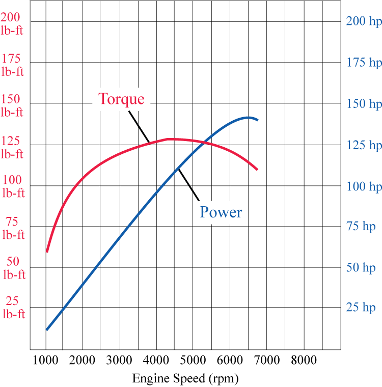
3. Suppose the graphs in Figure 1 show the torque and power curves of the 2015 and 2021 Brand X car models, respectively. Examine the curves and answer the questions below.

   

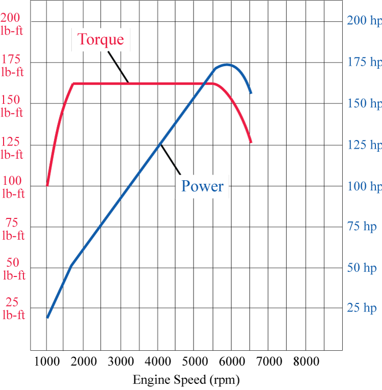
   A graph depicting the torque and power of the 2015 model car of brand X. The x-axis is labeled as Engine Speed (rpm) from 500 to 9000 by 500. The y-axis has two separate labels. The first label is associated with torque and is labeled from 0 pound-feet to 200 pound-feet by 25. The second label is associated with power and is labeled from 0 horsepower to 200 horsepower by 25. The graph for Torque starts at approximately (1000, 60), curves upward to peak at approximately (4500, 127), then curves downward to end at approximately (6750, 112). The graph for Power starts at approximately (1000, 12) and increases linearly until approximately (5500, 130) when its growth slows and begins curving, peaking at approximately (6500, 140) and curves downward to end at approximately (6750, 137).

   

   A graph depicting the torque and power of the 2021 model car of brand X using the same labels as the previous graph. The graph for Torque starts at (1000, 100) and rises sharply to approximately (1750, 162), remains constant to approximately (5500, 162), and curves gradually down ending at (6500, 127). The graph for Power starts at approximately (1000, 20), rises linearly to approximately (1700, 50), rises linearly at a different rate to approximately (5500, 170), then curves downward to end at approximately (5500, 155).

   1. Notice that in both graphs of Figure 1, the power curve intersects the torque curve at $5252\mathrm{rpm}$. Is that a coincidence? Explain.

   2. Use Figure 1a as well as the formula you obtained in Question 2c to estimate the horsepower range generated by the 2015 car's engine when the engine is revved from $2000$ to $3500\mathrm{rpm}$. (Answers will be approximate. Note that this is a typical rpm range in city traffic. Also notice how different your answer is from the "peak horsepower" rating typically advertised for consumers!)

   3. Repeat part b. for the 2021 edition of the car.

   4. From your answers above, which car would you expect to have better acceleration in typical city driving conditions?

   5. Summarize your findings in this problem by explaining why having a "flat" torque curve (as in the second illustration above) is advantageous in city driving. (This is typical with certain turbocharged or large displacement engines.)

4. Suppose a certain car's torque curve can be approximated by the function

   ${\rm T}\left(x\right)=200\sin {\displaystyle \frac{x}{3000}}$

   on the interval $\left(0,6500\right)$, where the independent variable x stands for rpm.

   1. Find a formula for the power function $P\left(x\right)$ (i.e., the horsepower as a function of engine speed) on the same interval.

   2. Use a graphing utility to graph the functions $T\left(x\right)$ and $P\left(x\right)$ on the interval $\left(500,6500\right)$.

   3. Suppose we accelerate the car (without shifting gears) from $0$ to $4000$ rpm in $4$ seconds. Assuming that the rate of change of the engine speed is constant, use your answer from part a. to express the engine's output in hp as a function of time (in seconds) during the acceleration (i.e., find the formula for $P\left(t\right)$).

   4. Convert your answer in part c. to kilowatts to obtain a formula for the engine's output in kilowatts as a function of time. Then use integration by parts to find the total work done by the engine, in kilojoules, during this acceleration run. (Hint: Use the formula from Question 1.)

5. 1. Suppose we accelerate the 2015 Brand X car model from $1000\mathrm{rpm}$ to $3500\mathrm{rpm}$ in $5$ seconds, without changing gears and while keeping the rate of change of engine speed constant. Use the Trapezoidal Rule and Figure 1a to estimate the work done by the engine. Express your answer in kilojoules. (Answers will be approximate.)

   2. Repeat part a. above for the 2021 Brand X car model, using Figure 1b.

   3. Explain why car performance enthusiasts and tuners often refer to torque or power curves by exclaiming, "I want as much area under the curve as possible."

   4. From your answers above, as well as those given to Question 3, would you prefer a "flat" or a "peaky" torque curve for city driving? Why? (There are no right or wrong answers.)

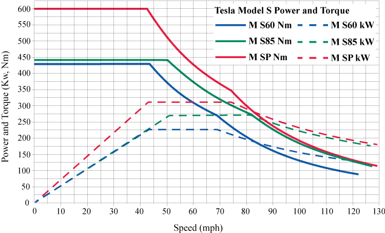
6. Figure 2 shows the torque and performance curves of various Tesla models.

   

   A graph of the power and torque of three Tesla car models, S60, S85, and SP. The x-axis is labeled Speed (mph), from 0 to 130 by 5. The y-axis is labeled Power and Torque (Kw, Nm), from 0 to 600 by 25.

   Tesla Model S60: The graph for torque starts at approximately (0, 425) and is constant until approximately (44, 425), curves gradually downward to approximately (68, 275), creating a slight cusp as it curves gradually downward further to end at approximately (122, 90). The graph for power starts at (0, 0) and rises linearly to approximately (43, 225), stays constant to approximately (68, 225), and curves gradually downward ending at approximately (122, 125).

   Tesla Model S85: The graph for torque starts at approximately (0, 440) and is constant until approximately (50, 440), curves gradually downward to approximately (82, 275), creating a slight cusp as it curves gradually downward further to end at approximately (127, 112). The graph for power starts at (0, 0) and rises linearly to approximately (51, 270), stays constant to approximately (82, 270), and curves gradually downward ending at approximately (127, 175).

   Tesla Model SP: The graph for torque starts at approximately (0, 600) and is constant until approximately (43, 600), curves gradually downward to approximately (74, 350), creating a slight cusp as it curves gradually downward further to end at approximately (129, 112). The graph for power starts at (0, 0) and rises linearly to approximately (43, 312), stays constant to approximately (74, 225), and curves gradually downward ending at approximately (129, 177).

   Source: Dr. Grzegorz Sieklucki, "An Investigation into the Induction Motor of Tesla Model S Vehicle"

   1. By visually examining the Tesla torque curves, explain the fundamental difference between them and those we discussed above.

   2. Based upon your observations about the graphs, explain why most electric cars have impressive acceleration in stop-and-go city traffic.

Creating a New Element

Recall from Section 3.7 our discussion of a chemical reaction where reactants A and B produce a new product substance C, a process represented by

$A+B\to C$.

In this project, we will derive and use a differential equation that describes such a process.

1. Suppose that in the above reaction for each gram of reactant A, b grams of B are used to form C. If we start with initial amounts $A_0$ and $B_0$, respectively, and $X\left(t\right)$ denotes in grams the amount of substance C already formed at time t, find the remaining amounts of reactants A and B at any time during the process.

2. Given that the rate of formation of substance C at any time is proportional to the product of the remaining amounts of reactants A and B, respectively, find a differential equation in terms of $X\left(t\right)$ that describes the process.

   (As in Question 1, let $A_0$ and $B_0$ stand for the initial amounts.)

3. Suppose a product substance C is being formed from reactant substances A and B and that for each gram of substance A, $3$ grams of B are used to form C. As in Question 1, let $X\left(t\right)$ denote the amount of C formed at time t, and assume that the initial amounts of reactants A and B are $A_0=60\text{grams}$ and $B_0=40\text{grams}$, respectively. Find the initial value problem describing this reaction. (Hint: Use your answer to Question 2.)

4. If $20$ grams of the product compound form during the first $5$ minutes, use the model you obtained in Question 3 to predict how much of the product compound C is present $10$ minutes into the process.

5. Use your model from Question 3 to predict what happens as $t\to \infty$. Interpret your answer.

A Sturdy Foundation

On November 7, 1940, the original Tacoma Narrows Bridge spectacularly collapsed under the sustained effect of strong and rhythmic wind forces. This stunning disaster was the result of what was then a poorly studied phenomenon called aeroelastic flutter caused by undamped periodic forces; its effect is closely related to what is called forced mechanical resonance.

Resonance might happen when a periodic external force is acting on an oscillating system. In this project, we will examine some conditions under which the phenomenon might occur, with the assumption that no damping forces are present. Such motion is called forced undamped motion.

1. The following initial value problem represents a spring-mass system where the oscillating mass m is acted upon by an external force as well as the restoring force of the spring it is attached to. In addition to k (the usual spring constant), f is also a constant.

   ${\displaystyle m\frac{{\mathit{d}}^{2}y}{\mathit{d}{t}^2}}+ky=f\sin \left(\theta t\right)$;   $y\left(0\right)=0$;   $y^{\prime }\left(0\right)=0$

   1. Compare the above IVP to that in Example 4 of Section 8.4 and describe any differences. Relate any mathematical differences to the forces acting on the oscillating mass.

   2. In words, describe why you would expect a major difference in the motion of a spring-mass system described by the above IVP, in contrast with Example 4 of Section 8.4. Are there any damping forces present?

   3. Find the period and frequency of the expression on the right-hand side of the differential equation.

2. 1. Find the general solution $y_c\left(t\right)$ of the associated homogeneous equation in the IVP above. Use the conventional notation $\omega =\sqrt{{\displaystyle \frac{k}{m}}}$.

   2. Starting with $y_p\left(t\right)=A\cos \left(\theta t\right)+B\sin \left(\theta t\right)$ as the initial guess, find a particular solution $y_p$ of the differential equation in Question 1. (Hint: See Exercises 39–44 and the preceding discussion in Section 8.4.)

   3. Use your answers to parts a. and b. as well as the initial conditions to find the solution $y\left(t\right)$ to the initial value problem of Question 1.

3. Find the formula for $Y\left(t\right)=\underset{\theta \to \omega }{\lim }y\left(t\right)$ (Hint: Use L'Hôpital's Rule.)

4. 1. Use the formula for $Y\left(t\right)$ that you obtained in Question 3 to examine $\underset{t\to \infty }{\lim }\left|Y\left(t\right)\right|$, and describe what happens to the amplitude of the oscillations when $\theta =\omega$ and t increases without bound.

   2. Use technology to obtain a graph that illustrates the behavior of $Y\left(t\right)$ as $t\to \infty$. (Choose your own values for the unspecified parameters. Answers will vary.)

   3. Use your answer to Question 4a (along with a limit argument) to explain the physical effect of $\theta$ approaching $\omega$ in this type of forced, undamped oscillating motion.

5. Your work on Question 4 and the answers you found provide mathematical insights into the physical phenomenon called resonance. This will occur in lightly damped or undamped systems when the frequency of the external driving force approaches the oscillating system's natural frequency, that is, when $\theta \to \omega$. Use your results to write a short paragraph explaining this phenomenon.

6. *There is actually a direct way to obtain $Y\left(t\right)$, that is, by finding the solution of the following initial value problem.

   ${\displaystyle m\frac{{\mathit{d}}^{2}y}{\mathit{d}{t}^2}}+ky=f\sin \left(\sqrt{{\displaystyle \frac{k}{m}}}t\right)$;  $y\left(0\right)=0$;  $y^{\prime }\left(0\right)=0$

   Find the solution of the IVP above to verify the formula for $Y\left(t\right)$ you obtained in Question 3b.

Curve Control

In this project, you will be introduced to a class of parametric curves called Bézier curves. They are important for their applications in engineering, computer graphics, and animation. This class of curves is named after Pierre Bézier (1910–1999), a design engineer for the French automaker Renault, who first demonstrated these curves’ use in designing automobile bodies in the 1960s. The design advantage of Bézier curves lies in the fact that they can easily be manipulated by moving around their so-called control points. In addition, it is easy to smoothly join together several Bézier curves for more complicated shapes.

1. The linear Bézier curve $B_{0,1}\left(t\right)$ from $P_0\left(a_0,b_0\right)$ to $P_1\left(a_1,b_1\right)$ is simply the line segment connecting the two points (note that $P_0$ and $P_1$ are the only control points in this case). Verify that this curve can be parametrized as

   $B_{0,1}\left(t\right)=\left(1-t\right)P_0+t{P}_1$, $t\in \left[0,1\right]$.

   and find $x\left(t\right)$ and $y\left(t\right)$ corresponding to this parametrization. (In this and subsequent questions, control points will be labeled $P_1\left(a_1,b_1\right)$, $0\le i\le 3$.)

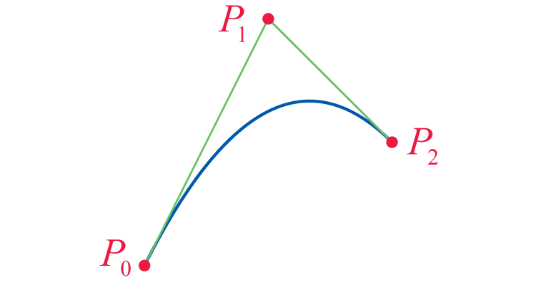
2. The Bézier curve $B_{0,1,2}\left(t\right)$ with control points $P_0$, $P_1$, and $P_2$ is a quadratic curve joining the points $P_0$ and $P_2$ in such a way that both line segments $\overline{P_0{P}_1}$ and $\overline{P_1{P}_2}$ are tangent to $B_{0,1,2}\left(t\right)$. Intuitively speaking, this means that the curve starts out at $P_0$ in the direction of $P_1$ and arrives at $P_2$ from the direction of $P_1$ (see Figure 1).

   Find $x\left(t\right)$ and $y\left(t\right)$ corresponding to the parametrization

   $B_{0,1,2}\left(t\right)=\left(1-t\right)B_{0,1}\left(t\right)+t{B}_{1,2}\left(t\right)$, $t\in \left[0,1\right]$

   and verify that $B_{0,1,2}\left(t\right)$ satisfies the conditions stated above.

   

   Three points labeled P₀, P₁, and P₂, moving from left to right and connected in sequence. P0 lies below the other two points, P1 lies above the other two points. A quadratic curve opening downward connects P0 and P2.

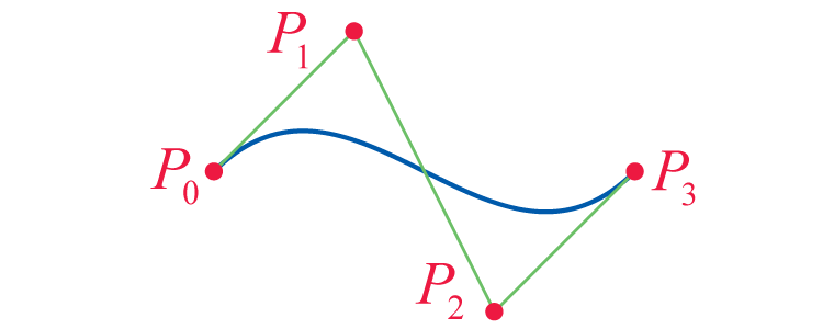
3. The cubic Bézier curve $B_{0,1,2,3}\left(t\right)$ with control points $P_0$, $P_1$, $P_2$, and $P_3$ joins $P_0$ and $P_3$ so that the line segments $\overline{P_0{P}_1}$ and $\overline{P_2{P}_3}$ are tangent to $B_{0,1,2,3}\left(t\right)$ at $P_0$ and $P_3$, respectively (see Figure 2). Verify that the following curve satisfies these conditions.

   $x\left(t\right)=a_0{\left(1-t\right)}^3+3a_1{\left(1-t\right)}^{2}t+3a_2\left(1-t\right)t^2+a_3{t}^3$

   $\phantom{t\in \left[0,1\right]}y\left(t\right)=b_0{\left(1-t\right)}^3+3b_1{\left(1-t\right)}^{2}t+3b_2\left(1-t\right)t^2+b_3{t}^3$, $t\in \left[0,1\right]$

   

   Four points labeled P₀, P₁, P₂, and P₃, moving from left to right and connected in sequence. P1 lies above the other three points, P2 lies below the other three points. P₀ and P₁ are at the same height. A cubic curve connects P₀ and P₃, curving upwards towards P₂ and curving downwards towards P₃.

4. Show that the parametrization in Question 3 corresponds to

   $B_{0,1,2,3}\left(t\right)=\left(1-t\right)B_{0,1,2}\left(t\right)+t{B}_{1,2,3}\left(t\right)$.

5. Use Question 3 to verify that the Bézier curve with control points $P_0\left(1,3\right)$, $P_1\left(3,7\right)$, $P_2\left(6,9\right)$, and $P_3\left(8,6\right)$ has the following parametrization

   $x\left(t\right)=-2t^3+3t^2+6t+1$

   $y\left(t\right)=-3t^3-6t^2+12t+3$

6. Find the slope of the curve in Question 5 at

   1. $t=0$,

   2. $t={\displaystyle \frac{1}{2}}$,

   3. $t=1$

7. Use a computer algebra system to graph the Bézier curve of Question 5 along with its control points. If your CAS has animation capabilities, explore what happens if you move around the control points in the plane.

Keeping Time Is Timeless

In this project, we will examine a pendulum that uses the solution of the tautochrone problem discussed in Section 9.1. Such a pendulum was invented as early as 1657 by the Dutch mathematician, physicist, and astronomer Christiaan Huygens (1629–1695). Huygens was interested in developing accurate clocks, and thus needed a pendulum whose period of oscillation was independent of amplitude (i.e., unaffected by the initial position of the pendulum bob when released to swing freely). Huygens' work, Horologium Oscillatorium (published in 1673) as well as his numerous other groundbreaking findings in various areas of mathematics, physics, engineering, and astronomy, are a testament to his brilliance and creativity. We will analyze his invention by appropriately modifying the parametric equations of the cycloid introduced in Example 4 of Section 9.1.

1. 1. Sketch the inverted cycloid traced out by a point P on a circle of radius a that rolls counterclockwise along the line $y=2a$ assuming that P starts out at $\left(0,2a\right)$. (The circle is positioned between the x-axis and $y=2a$.) Show the path traced out by P after two full revolutions; that is, sketch the cycloid on the parametric interval $0\le \theta \le 4\pi$.

   2. Make a sketch to show the inverted cycloid of part a. on the parametric interval $-\pi \le \theta \le \pi$.

2. 1. Find the parametric equations of the inverted cycloid (henceforth referred to simply as cycloid) in Question 1.

   2. Use technology to reproduce the graph you sketched in Question 1b.

3. Now, suppose we create a pendulum by attaching a cord of length $4a$ to the cusp located at $\left(0,2a\right)$ of the cycloid of Question 1b, and let the bob swing left and right, partially wrapping the cord around the cycloid in the process (see Figure 1).

   

   An unlabled cartesian plane. A dashed semi-circle lies beneath the x-axis ranging from quadrant 3 to quadrant 4. Quadrants 1 and 2 both contain a quarter-circle, starting at the end points of the semi-circle, curving inward towards the origin, and meeting at a cusp on the y-axis. In quardrant 1, a section from the cusp to a point labeled Q is highlighted on the quarter-circle. A line then extends from point Q to an unlabeled point on the semi-circle in quadrant 4.

   Source: Wolfram Demonstrations Project

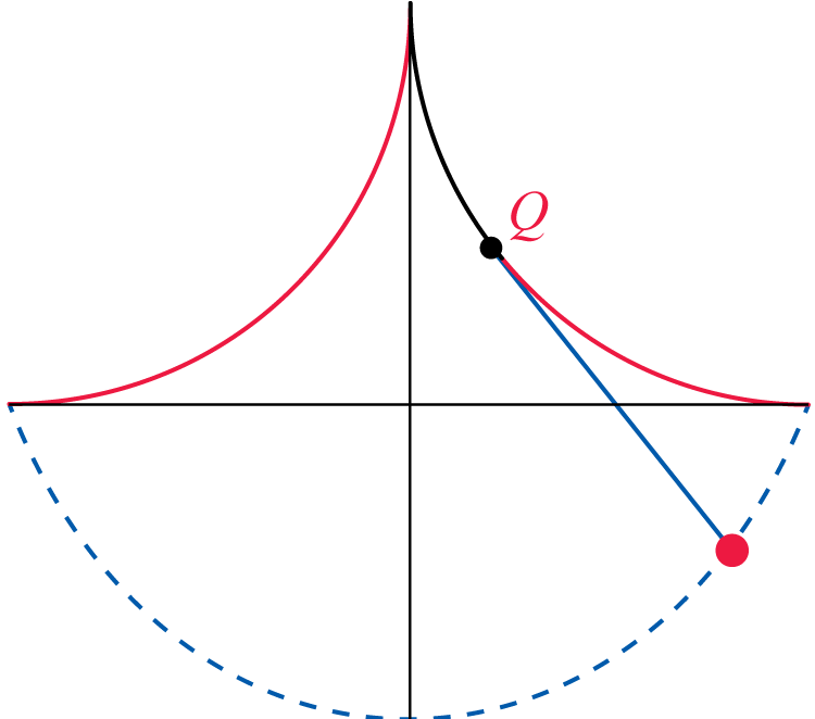
   1. Given that the length of the cord is equal to $4a$, where does the bob touch the cycloid at the pendulum's most extreme positions? That is, what is the location of the bob when the cord is completely wrapped around the cycloid? (Hint: See Example 7 in Section 9.2.)

   2. Note that while the pendulum is moving, the "free" part of the cord (the portion that is not wrapped around the cycloid) is tangent to the cycloid. Let Q denote the point of tangency (see Figure 1), and suppose that Q corresponds to the parameter value ${\theta }_0$. Find the length s of the portion of the cord that is wrapped around the cycloid under these conditions. (Hint: Make a detailed sketch and consider the angle that the tangent of the cycloid forms with the x-axis. See Exercise 71 in Section 9.2.)

4. 1. Use your work on Question 3b to obtain a parametrization of the path traced out by the bob of the pendulum. (Hint: First find x and y in terms of $\theta$ and s; then eliminate s by making use of the formula you found in Question 3b.)

   2. What kind of parametric curve have you obtained in part a.? Use your answer to conclude that the cycloidal pendulum is tautochronous; that is, its period of oscillation is independent of amplitude. (See the discussion and derivation under Topic 2 in Section 9.1.)

Working in Harmony

In this project, we are going to expand on our earlier work with the harmonic series. In the process, we will meet a famous constant called Euler's constant, also known as the Euler-Mascheroni constant. (This number is not to be confused with $e\approx 2.71828$, the natural base, which is also known as Euler's number.)

1. As in Example 6 of Section 10.2, we let $s_n$ stand for the n^th partial sum of the harmonic series; that is,

   $s_n=1+{\displaystyle \frac{1}{2}}+\cdots +{\displaystyle \frac{1}{n}}$.

   (The partial sum $s_n$ is also called the n^th harmonic number.) For each $n\ge 1$, we define

   $d_n=s_n-lnn$.

   Prove that $d_n>0$ for any positive integer n. (Hint: Refer to the illustration provided for Exercise 65 of Section 10.2, and start by comparing $s_n$ with ${\displaystyle {\int }_1^{n+1}\left({\displaystyle \frac{1}{x}}\right)\mathit{d}x}$.)

2. Prove that $\left\{d_n\right\}$ is a decreasing sequence. (Hint: Referring again to the figure from Exercise 65 of Section 10.2, fix an n and identify a region whose area is $d_n-d_{n+1}$ .)

3. Use an appropriate theorem from the text to show that the sequence $\left\{d_n\right\}$ is convergent. Letting $\gamma =\underset{n\to \infty }{\lim }{d}_n$, this limit is called Euler's constant. It is important in many applications throughout various areas of mathematics, and like other famous constants (including π and e) can be approximated with great precision using modern computing power. Surprisingly, however, it is not yet known whether γ is rational or irrational!

4. Use the convergence of $\left\{d_n\right\}$ to prove that the sequence $a_n={\displaystyle \sum _{i=n}^{2n}{\displaystyle \frac{1}{i}}}$ converges and find its limit.

5. Use a computer algebra system to approximate γ, accurate to the first $10$ decimal places.

6. Use the approximate value of γ found in Question 5 to estimate $s_n$, rounded to $5$ decimal places, for a. $n=\mathrm{10,000}$ and b. $n=\mathrm{2,000,000}$. Compare the latter estimate with the answer for Exercise 125b of the Chapter 10 Review.

A Spoonful of Sugar

In this project, you will build a model that sheds light on the mathematics behind medicine dosage. Your knowledge of sequences and exponential decay will be essential for this work. It is important to note, however, that pharmacology is a complicated science, and numerous factors are taken into consideration when actual drug dosage for the treatment of a particular condition is determined. The model in this project, while it illustrates the basic ideas behind drug dosage, should not be used in real-life situations.

1. Clinical experiments have shown that the concentration $C\left(t\right)$ of a drug in the bloodstream decays at a rate proportional to the instantaneous level of concentration.

   1. Using k for the constant of proportionality and assuming an initial level of concentration $C\left(0\right)=D$, set up an initial value problem to find $C\left(t\right)$. Assume t is measured in hours.

   2. Solve your initial value problem to find a formula for $C\left(t\right)$.

2. 1. Starting with a concentration level of $C\left(0\right)=D$, another dose is administered after a dosage period of p hours that raises the concentration level by D. Construct a formula for the level of concentration just before the new dose is administered, and denote it by $C_1$. The reason for this naming convention is that this is the concentration level just before the first so-called maintenance dose is administered. Note, however, that in practice the initial, so-called loading dose, and the maintenance dose are usually different. (Hint: Note that $C_1=C\left(p\right)$.)

   2. After yet another period of p hours, the same dosage D is administered again. Find the level of concentration just before this second maintenance dose and denote it by $C_2$.

3. Iterating the process in Question 2, find a formula for $C_n$, $n\ge 2$. (Hint: Use the formula for the sum of a finite sequence.)

4. Find $C=\underset{n\to \infty }{\lim }{C}_n$ to determine the long-term concentration after many repeated doses.

   The minimum concentration at which a drug is effective is often abbreviated as MEC (for minimum effective concentration). In this project, we will denote that concentration by $m_e$. On the other extreme, above a certain concentration level, a drug will typically cause unwanted side effects and is said to be toxic. This concentration level is often referred to as the MTC (for minimum toxic concentration), and we will denote it by $m_t$. The interval $\left[m_e,m_t\right]$ is called the therapeutic window. In order for a given drug to work, that is, to achieve the desired therapeutic effects without causing harm, we need to keep its concentration level in this interval.

   Now suppose we want to prescribe a dosage amount with an optimal dosage period that keeps the drug concentration within the therapeutic window for the duration of treatment. One possible approach is to try to maximize the time between subsequent doses for the patient's convenience. In order to achieve that, we administer a loading dose that raises the concentration level to just below $m_t$, the top of the therapeutic window. Then we wait until the concentration drops down to $m_e$ and administer a maintenance dose that raises the concentration by $D_m=m_t-m_e$ to bring the concentration level back to (near) $m_t$. In other words, the goal is to achieve a long-term concentration $C=m_e$ with repeated maintenance doses $D_m$. In Question 5, we will determine the dosage interval to achieve this.

5. Substitute $C=m_e$ and $D=m_t-m_e$ into the formula you obtained for C in your answer to Question 4, and then solve for p to obtain a formula for the optimal dosage interval.

6. Suppose that a certain medication's therapeutic window ranges from a concentration of $150$ nanograms per milliliter (${\displaystyle \frac{\mathrm{ng}}{\mathrm{mL}}}$) to $600{\displaystyle \frac{\mathrm{ng}}{\mathrm{mL}}}$ and that its half-life is $12$ hours. Suppose one tablet raises the concentration by $150{\displaystyle \frac{\mathrm{ng}}{\mathrm{mL}}}$. (A nanogram is one-billionth of a gram.)

   1. What loading dose of this drug would your model recommend?

   2. Based on your work on Question 5, what would be the optimal dosage and dosage interval for this drug? (Hint: Recall the definition of half-life from Exercises 66–67 in Section 1.2.)

Planes, Vectors, and Quadrilaterals

In this project, we are going to use vectors to prove an interesting property of quadrilaterals. In fact, the result is general enough that our quadrilateral doesn’t have to be planar, in other words, its vertices do not have to lie in the same plane!

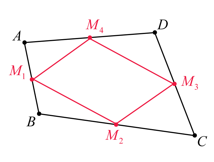
1. Let A, B, C, D be four points in ${\mathrm{ℝ}}^3$, with $M_1$, $M_2$, $M_3$, and $M_4$ being the midpoints of the line segments $\stackrel{-}{AB}$, $\stackrel{-}{BC}$, $\stackrel{-}{CD}$, and $\stackrel{-}{DA}$, respectively. Consider the vector $\overrightarrow{M_1{M}_2}$ and show that

   $\overrightarrow{M_1{M}_2}={\displaystyle \frac{1}{2}}\left(\overrightarrow{AB}+\overrightarrow{BC}\right)$.

   

2. Prove a statement analogous to the one in Question 1 for the vector $\overrightarrow{M_3{M}_4}$ and show that

   $\overrightarrow{M_1{M}_2}=-\overrightarrow{M_3{M}_4}$.

3. Using the results of Questions 1 and 2, argue that the quadrilateral $M_1{M}_2{M}_3{M}_4$ is a parallelogram.

4. Explain why the proof of Question 3 does not require that the points A, B, C, and D lie in the same plane.

5. Use vectors in the three‑dimensional coordinate system to prove the statement of Question 3: If ABCD is a (not necessarily planar) quadrilateral in ${\mathrm{ℝ}}^3$, then the midpoints of its sides determine a parallelogram. (Hint: To simplify your calculations, you can assume that three of the vertices lie in the same coordinate plane with one of them, say A, located at the origin, and an adjacent vertex, such as B, lying on a coordinate axis.)

The Pipe of Least Resistance

In this project, we will use calculus to provide an introduction into the study of the velocity of a fluid flowing in a circular pipe. This will provide a glimpse into the very complex area of study called fluid dynamics. In the Chapter 14 Application Project, we will expand on our results and use them to better understand blood flow in human blood vessels.

Circular pipes (i.e., pipes with circular cross-sections) are most often used in practical applications, such as city water systems, oil transportation lines, automotive cooling systems, etc. because they are the best at withstanding distortions caused by large differences between interior and exterior pressures.

We will distinguish between laminar and turbulent flows. Laminar flow is smooth, streamlined flow where fluid particles travel along smooth, observable paths called streamlines that don't cross each other. Fluid layers flow over one another without mixing. Turbulent flow, on the other hand, is characterized by fluid layers crossing paths, particles traveling along irregular trajectories, and the presence of a multitude of small, chaotic whirlpool-like swirls (also called eddies) that disturb and slow down the flow, absorbing a lot of energy. Turbulence can be observed, for example, in the flow of rivers, or in the way smoke rises from a chimney. It is important to note that, due to friction and other factors, no flow is purely turbulent or purely laminar. In fact, no matter what the flow type, there is always some internal friction, or resistance to flow, between adjacent layers of fluid, called viscosity. A famous researcher who pioneered the study of fluid flow was British engineer Osborne Reynolds (1842–1912). He studied streamlines by injecting dye into fluid flowing in a glass pipe. The characteristic of a fluid known as the Reynolds number, denoted Re, was named after him. The Reynolds number is the ratio of inertial forces to viscous forces in flowing fluid. Below the value of $\mathrm{Re}=2300$, the flow in a circular pipe is considered laminar; for $2300\le \mathrm{Re}\le 4000$, it is called transitional; while above 4000, it becomes turbulent. (Note, however, that these numbers are not absolute. Some consider the flow to be transitional above $\mathrm{Re}=2100$.)

In this project, we will assume that the flow is laminar, and fully developed. This means that the pipe is long enough, and the flow takes place far enough from entry into the pipe, so that the entrance effects are negligible. The velocity of each fluid particle is constant and parallel to the axis of the pipe, and velocity depends only on the distance from the axis, which we will denote by r. We will assume that the fluid is incompressible, that is, neither its volume nor its density changes with pressure. We will further assume that the fluid completely fills the interior of the tube and that the flow is driven by pressure difference. The pipe is assumed to be horizontal, so the effects of gravity won't be considered. Lastly, we will also assume the so-called no-slip condition, which is that the outer layer of the fluid—the layer that is in direct contact with the surface of the pipe—has zero velocity. As a result, the closer the fluid is to the axis of the tube, the greater its flow velocity, with the maximum occurring along the axis of symmetry of the tube. This maximum velocity is commonly called centerline velocity in fluid dynamics. The phenomenon just described is the result of friction, or viscosity. As a first task, we will show that for a fully developed laminar flow, the curve formed by the endpoints of the flow velocity vectors is a parabola. This is called the velocity profile of the flow (see Figure 1). Note that by our assumptions, the velocity profile for fully developed laminar flow remains unchanged in the direction of flow.

We note that the scenario just described is one of the few special cases when it is actually possible to obtain theoretical results. In the case of more chaotic or turbulent flows, one must resort to empirical results produced by experiments under carefully controlled laboratory conditions.

A parabola opening towards the left bordered on the top and bottom by the pipe wall. Horizontal vector arrows extend from left to right, pointing towards the curve of the parabola.

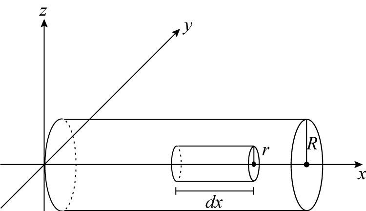
1. Suppose that a circular pipe of radius R is positioned in the three-dimensional coordinate system so that its axis of symmetry coincides with the x-axis. Find the equation of the surface of the pipe.

In order to understand how the velocity of the flow depends on the distance from the axis, we will consider a small differential volume element in the form of a circular cylinder around the x-axis and in the axial direction, with base radius r and length $\mathit{d}x$ (see Figure 2).

A three dimensional space with two cylinders centered around the x-axis. The larger cylinder has a labeled radius of R. The smaller cylinder has a labled radius of r and a length of $dx$.

Assuming flow in the positive direction, the volume element illustrated in Figure 2 will move because the fluid pressure acting on its left base is greater than that on its right base. On the other hand, a restraining force arising from the fluid's internal friction, or viscosity, is acting in the direction opposite of movement. In general, the force restraining the movement of a layer of fluid by the layer next to it is proportional to their area of contact A and the change of velocity from one layer to the other, divided by the distance over which this change is occurring. In our case,

$F_r=\eta A\cdot {\displaystyle \frac{\mathit{d}v}{\mathit{d}r}}$,

where the constant of proportionality $\eta$ (the Greek letter eta) is called the coefficient of viscosity. In general, the thicker a fluid is, the more viscous it is, with a corresponding higher $\eta$-value. For example, syrup is more viscous than water, motor oil is more viscous than cooking oil, etc.

2. 1. Denoting fluid pressures acting on the two bases of the differential volume element in Figure 2 by P and $P-\mathit{d}P$, respectively, show that the force acting in the positive direction on the volume element is

      $F=\pi r^2\mathit{d}P$.

      (Hint: Remember that $P={\displaystyle \frac{F}{A}}$.)

   2. Show that the restraining force arising from viscosity is

      $F_r=2\pi r\cdot \mathit{d}x\cdot \eta \cdot {\displaystyle \frac{\mathit{d}v}{\mathit{d}r}}$.

   3. Use parts a. and b. to obtain the equation of motion for the volume element. (Hint: Apply Newton's Second Law of Motion, and remember that we are assuming each differential volume element is moving with constant velocity, so its acceleration is zero.)

3. 1. Use the equation of motion you obtained in Question 2c to show that

      $\mathit{d}v={\displaystyle \frac{1}{2\eta }}\cdot {\displaystyle \frac{\mathit{d}P}{\mathit{d}x}}r\mathit{d}r$.

   2. Integrate the above equation to find a formula for $v\left(r\right)$. (Hint: Because the flow is fully developed, ${\displaystyle \frac{\mathit{d}P}{\mathit{d}x}}$ is constant. Don't forget about the constant of integration.)

4. 1. Use the no-slip condition (i.e., the condition $v\left(R\right)=0$) to find the value of the constant of integration in your answer to Question 3b, and verify the formula

      $v\left(r\right)=-{\displaystyle \frac{R^2}{4\eta }}\cdot {\displaystyle \frac{\mathit{d}P}{\mathit{d}x}}\left(1-{\displaystyle \frac{r^2}{R^2}}\right)$.

      (Note that since $v\left(r\right)$ is positive, our formula reflects the fact that ${\displaystyle \frac{\mathit{d}P}{\mathit{d}x}}$ is negative, meaning pressure drops in the direction of flow.)

   2. Given that flow velocity reaches its maximum along the axis (i.e., $v_{\max }=v\left(0\right)$ ), show that

      $v\left(r\right)=v_{\max }\left(1-{\displaystyle \frac{r^2}{R^2}}\right)$.

   3. Conclude that the velocity profile of a fully developed laminar flow is parabolic.

5. Suppose that the centerline speed of a fully developed laminar flow in a circular tube of radius $3\mathrm{cm}$ is $10{\displaystyle \frac{\mathrm{cm}}{\mathrm{s}}}$. Find the equation of the parabola that represents the velocity profile of this flow. (Hint: Place the parabola in the usual xy-system, with its vertex at the origin and opening leftward. Let the vector $v=〈10,0,0〉$ represent a velocity of $10{\displaystyle \frac{\mathrm{cm}}{\mathrm{s}}}$.)

6. If the flow is more turbulent, experiments show that the equation

   $v\left(r\right)=v_{\max }{\left(1-{\displaystyle \frac{r^2}{R^2}}\right)}^{{\displaystyle \frac{1}{p}}}$  ($p>1$)

   better models the fluid velocity within the pipe. For example, $p=7$ provides a fairly accurate model for certain turbulent flows. By choosing appropriate values for r, R, and $v_{\max }$, graph a velocity profile for such a flow. (Answers will vary.)

A Satellite in Motion Stays in Motion

Some orbits, such as for certain Earth satellites, can be fairly closely approximated by circles. The slight loss of accuracy in doing so is often well justified by the gain in simplicity of certain calculations. In this project, you will be guided to prove Kepler's Second and Third Laws in the case when circular orbits are assumed.

Let us now assume that a satellite is orbiting along a circular path of radius R. As we did in Section 12.4, we will start by combining Newton's Law of Universal Gravitation with his Second Law of Motion to obtain the equation of motion:

$\mathbf{F}=m{\mathbf{r}}^{″}=m\mathbf{a}=-{\displaystyle \frac{GMm}{r^3}}\mathbf{r}$.

1. 1. Assume that the satellite's position function is $\mathbf{r}\left(t\right)=⟨r\left(t\right)\cos \left(\theta \left(t\right)\right),r\left(t\right)\sin \left(\theta \left(t\right)\right)⟩$, where by assumption, $r\left(t\right)=R$. Recall the unit vectors $\mathbf{u}\left(t\right)=⟨\cos \left(\theta \left(t\right)\right),\sin \left(\theta \left(t\right)\right)⟩$ and ${\mathbf{u}}_{\perp }\left(t\right)=⟨-\sin \left(\theta \left(t\right)\right),\cos \left(\theta \left(t\right)\right)⟩$ that we used in Section 12.4, Topic 1 to describe the motion in terms of polar variables r and θ of an object with position function

      $\mathbf{r}\left(t\right)=⟨r\left(t\right)\cos \left(\theta \left(t\right)\right),r\left(t\right)\sin \left(\theta \left(t\right)\right)⟩$.

      Explain why, in our case, $\mathbf{F}\cdot {\mathbf{u}}_{\perp }=0$.

   2. Use the above observations and the fact that $r\left(t\right)$ is constant to prove that

      $r\left(t\right){\theta }^{″}\left(t\right)=0$.

2. 1. Use your work above to conclude that the angular velocity

      $\omega ={\displaystyle \frac{\mathit{d}\theta }{\mathit{d}t}}$

      of the orbiting satellite is constant.

   2. Find the formula for ${\displaystyle \frac{\mathit{d}A}{\mathit{d}t}}$ in terms of $\omega$ and deduce Kepler's Second Law from the observation made in part a.

3. Use the normal component of acceleration and the curvature of the circular path (Section 12.3, Example 4) along with Newton's Second Law of Motion to show

   ${\displaystyle \frac{GM}{R^2}}=R{\omega }^2$.

4. 1. Use the above result to show that the period T can be expressed as

      $T={\displaystyle \frac{2\pi }{\omega }}$,

   2. By calculating ${\displaystyle \frac{T^2}{R^3}}$, use part a. to finish the proof of Kepler's Third Law.

Basketball Scoring

In this project you will use vector functions to develop a simple model for three-point basketball shots. To keep the model simple, we will be ignoring air resistance, friction, and other forces. Furthermore, by “scoring,” we will mean that the ball falls straight into the basket on its way downward (i.e., we will ignore the possibility of the ball bouncing in off the backboard, or any energy losses as a result of spins, etc.). For further studies, or for more refined models, the interested student should consult resources such as John Fontanella's book, The Physics of Basketball.

1. A basketball player is attempting a three‑pointer from a horizontal distance of $24.7\text{feet}$. He is releasing the ball from $7\text{feet}$ above ground level, aimed directly toward the basket at an angle of elevation of $45°$, with an initial velocity of $v_0$. Supposing that the player stands at the origin and the basket is in the positive y‑direction, use the three‑dimensional coordinate system to find a vector function describing the position of the ball after release as a function of time. (Assume one unit on each axis corresponds to a distance of $1$ foot.)

2. Use your answer to Question 1 to verify that the basketball's trajectory is a parabola.

3. Assuming a standard hoop height of $10\text{feet}$, find the initial speed for the ball that ensures that the player described in Question 1 scores.

4. Use your answer from Question 3 to find the necessary initial velocity vector for the basketball if the player is to score from the same spot (i.e., the origin) but this time, shooting while running along the line $y=x$ at a speed of $10\mathrm{mph}$ in the positive direction.

5. Find a formula for and graph the required initial speed as a function of the angle of elevation over the interval $\left(0,{\displaystyle \frac{\pi }{2}}\right)$ if the player is to score (assuming the same spot and release height as in Question 1).

6. Generalizing your work on Question 5, find a formula for the initial speed of a successful shot if the player stands d feet from the hoop and shoots at an angle α upward from horizontal, with a release height of h feet.

Exactly the Difference

In this project you will use your experience with partial derivatives and differentials to learn how to solve an important class of differential equations, called exact equations. Ordinary differential equations of this type are noted for their widespread applications in physics and engineering. (See Section 8.1 for the definitions of differential equation and solution. Other than the basic definitions, this project does not directly rely on, and can be considered independently of Chapter 8.)

1. Suppose that the first‑order partial derivatives of the function $z=f\left(x,y\right)$, are both continuous on a region R. If c is a constant and $y=y\left(x\right)$ is defined implicitly by the equation $f\left(x,y\right)=c$, show that y solves the differential equation

   $f_y\left(x,y\right)\cdot y\prime =-f_x\left(x,y\right)$.

2. Now consider a differential equation of the form

   $M\left(x,y\right)\mathit{d}x+N\left(x,y\right)\mathit{d}y=0$  (1)

   and assume that there is a two‑variable function $f\left(x,y\right)$ such that

   ${\displaystyle \frac{\partial f\left(x,y\right)}{\partial x}}=M\left(x,y\right)$  and  ${\displaystyle \frac{\partial f\left(x,y\right)}{\partial y}}=N\left(x,y\right)$

   (such a differential equation is called exact, while $f\left(x,y\right)$ is called a potential function). Use your answer to Question 1 to show that the set of level curves $f\left(x,y\right)=C$, $C\in \mathrm{ℝ}$ form a family of solutions of the differential equation (1).

3. Suppose that $M\left(x,y\right)$ and $N\left(x,y\right)$, as well as their first‑order partial derivatives, are continuous on an open region R. Show that a necessary condition for equation (1) to be exact is the following equality.

   ${\displaystyle \frac{\partial M\left(x,y\right)}{\partial y}}={\displaystyle \frac{\partial N\left(x,y\right)}{\partial x}}$

   (Note: If we require a bit more of R, the above condition is also sufficient for exactness, a statement we will not rigorously prove here, but the construction of a potential function under the stated conditions is outlined in Questions 5 and 6.)

4. Use Question 3 to determine which of the following equations is exact.

   1. $\left(2x+y{e}^{xy}\right)\mathit{d}x+\left(x{e}^{xy}-1\right)\mathit{d}y=0$

   2. $\left(3x^{2}y-{\displaystyle \frac{1}{\sqrt{x}}}\right)\mathit{d}x+\left(x^3-\sqrt{x}\right)\mathit{d}y=0$

5. Explain why the potential function f of an exact equation must satisfy

   $f\left(x,y\right)={\displaystyle \int M\left(x,y\right)\mathit{d}x}+g\left(y\right)$,

   where g is some function of the variable y.

6. Show that if the equation (1) is exact, then the equality

   $N\left(x,y\right)={\displaystyle \frac{\partial }{\partial y}}{\displaystyle \int M\left(x,y\right)\mathit{d}x}+g^{\prime }\left(y\right)$,

   must hold.

7. Use Questions 5 and 6 to solve the equation $2\left(x-y^2\right)\mathit{d}x+y\left(9y-4x\right)\mathit{d}y=0$ by determining its potential function $f\left(x,y\right)$ and identifying the family of solutions as $f\left(x,y\right)=C$. (Hint: After identifying $M\left(x,y\right)$ and $N\left(x,y\right)$, use Question 5 to obtain a tentative formula for $f\left(x,y\right)$, then use Question 6 to determine the unknown function $g\left(y\right)$.)

8. Verify that the equation $\left(2+x\right)y\mathit{d}x+2x\mathit{d}y=0$ becomes exact after multiplying by the integrating factor $I\left(x,y\right)=xy{e}^x$. Solve the resulting equation.

Houston, We Have Liftoff!

In the Chapter 6 Application Project, we derived the velocity function for a rocket that is applicable to its first few moments after blastoff. Our analysis assumed that gravity during the first few moments can be considered to be constant and, at the same time, is an important factor in determining the rocket’s velocity. That velocity function can be expressed as

$v\left(t\right)=v_e\ln {\displaystyle \frac{m_0}{m\left(t\right)}}-gt$,   (1)

where $v_e$ is the (positive) magnitude of the relative exhaust velocity of the expelled gas, $m_0$ is the initial total mass of the rocket (including fuel), $m\left(t\right)$ is the combined mass of the rocket and fuel at time t, and g is the acceleration due to gravity. After the initial blastoff phase, drag due to gravity is a less important factor in calculating change in velocity, and equation (1) is often reduced to

$\Delta v=v_e\ln {\displaystyle \frac{m_0}{m_f}}$,   (2)

where $\Delta v$ represents the change in velocity over a period in which fuel is burned and the combined mass of the rocket and fuel is reduced from $m_0$ to $m_f$. Equation (2) is the classic rocket propulsion equation that was derived independently by the Russian rocket scientist Konstantin Tsiolkovsky, the American Robert H. Goddard, and the German Hermann Oberth in the first couple decades of the 20^th century, and also in the early 19^th century by the British mathematician William Moore.

In modern practice, booster rockets are often used to overcome drag due to gravity and atmospheric resistance in the initial blastoff phase, after which they are jettisoned. The booster rockets are attached to the sides of a central stacked column of rocket stages, each of which is also jettisoned in sequence until only the payload remains, with the goal of accelerating the payload to a final desired velocity $v_f$. Rocket stages (and booster rockets) are used so that the mass of the remaining rocket can be decreased as each stage is detached.

In this project, you will derive a formula for the relative masses of each stage of a two-stage rocket given the goal of minimizing total mass and achieving a given final velocity for the payload. We will assume that gravitational and atmospheric drag factors are overcome by booster rockets, and hence that only equation (2) need be considered in designing the central stack consisting of two stages and a payload.

1. Let $m_1$ and $m_2$ denote the masses of, respectively, the first and second stages of the rocket when they are filled with fuel, and let P be the mass of the payload. Assume that the mass of each stage, when emptied of fuel, is the product of a structural factor s and its fuel-filled mass, where s is a positive number between $0$ and $1$ (s is typically less than $0.1$). Then the initial mass of the stack consisting of two stages and payload is $m_1+m_2+P$, and the mass after the fuel of stage 1 is expended is $s{m}_1+m_2+P$. Similarly, after stage 1 is jettisoned, the initial mass of the stack consisting of stage 2 and payload is $m_2+P$ and its mass after the fuel of stage 2 is expended is $s{m}_2+P$. If we let $\Delta v_1$ denote the change in velocity of the initial stack due to the fuel of stage 1 being burned, and $\Delta v_2$ the change in velocity of the second stage and payload due to the fuel of stage 2 being burned, then the final velocity achieved by the payload is $v_f=\Delta v_1+\Delta v_2$. Use these labels and equation (2) to express $v_f$ as a function of $m_1$, $m_2$, s, $v_e$, and P. Name the function you construct g, and since $m_1$ and $m_2$ are the two quantities we are free to vary, we will consider g to be a function of the variables $m_1$ and $m_2$.

2. Our goal is to minimize the function $f\left(m_1,m_2\right)=m_1+m_2+P$ subject to the constraint $g\left(m_1,m_2\right)=v_f$, and we will use the method of Lagrange multipliers to do so. The method is difficult to apply to f and g as originally defined, but it becomes much more tractable if we make a change of variables. To that end, let

   $n_1={\displaystyle \frac{m_1+m_2+P}{s{m}_1+m_2+P}}$  and  $n_2={\displaystyle \frac{m_2+P}{s{m}_2+P}}$.

   With these definitions, show that

   ${\displaystyle \frac{\left(1-s\right)n_1}{1-s{n}_1}}={\displaystyle \frac{m_1+m_2+P}{m_2+P}}$  and  ${\displaystyle \frac{\left(1-s\right)n_2}{1-s{n}_2}}={\displaystyle \frac{m_2+P}{P}}$,

   and consequently that

   $\begin{array}{l}{\displaystyle \frac{m_1+m_2+P}{P}}=\left({\displaystyle \frac{m_1+m_2+P}{m_2+P}}\right)\left({\displaystyle \frac{m_2+P}{P}}\right)\\ \phantom{{\displaystyle \frac{m_1+m_2+P}{P}}}={\displaystyle \frac{{\left(1-s\right)}^2{n}_1{n}_2}{\left(1-s{n}_1\right)\left(1-s{n}_2\right)}}\end{array}$.

3. Note that an ordered pair $\left(\widetilde{m_1},\widetilde{m_2}\right)$ that minimizes the function $f\left(m_1,m_2\right)=m_1+m_2+P$ will minimize the expression ${\displaystyle \frac{m_1+m_2+P}{P}}$, and hence will also simultaneously minimize the expression $\ln {\displaystyle \frac{m_1+m_2+P}{P}}$. The reasoning behind this is identical to the observation in Examples 3 and 4 of Section 13.8 that minimizing the square of a given distance function simultaneously minimizes the original distance function. Consequently, and because it makes the task easier, we will minimize the expression $\ln {\displaystyle \frac{m_1+m_2+P}{P}}$, which means we will minimize $\hat{f}\left(n_1,n_2\right)=\ln {\displaystyle \frac{m_1+m_2+P}{P}}=\ln {\displaystyle \frac{{\left(1-s\right)}^2{n}_1{n}_2}{\left(1-s{n}_1\right)\left(1-s{n}_2\right)}}$ subject to the constraint $g\left(n_1,n_2\right)=v_e\ln \left(n_1\right)+v_e\ln \left(n_2\right)=v_f$. Use the method of Lagrange multipliers to show that the minimum of $\hat{f}$ occurs when

   $n_1=n_2=e^{{\displaystyle \frac{v_f}{2v_e}}}$.

   (Hint: Use properties of logarithms to rewrite $\hat{f}$ before differentiating.)

4. Show that $m_2=\left({\displaystyle \frac{n_2-1}{1-s{n}_2}}\right)P$ and that $m_1=\left({\displaystyle \frac{n_1-1}{1-s{n}_1}}\right)\left(m_2+P\right)$.

5. The Falcon 9 two-stage rocket by SpaceX is capable of lifting a payload of approximately $23$ metric tons to low Earth orbit. Assuming a structural factor $s=0.04$, exhaust velocity $v_e=3.5{\displaystyle \frac{\mathrm{km}}{\mathrm{s}}}$, and final velocity $v_f=10{\displaystyle \frac{\mathrm{km}}{\mathrm{s}}}$, determine $m_1$ and $m_2$.

Sources:en.wikipedia.org/wiki/Tsiolkovsky_rocket_equation; en.wikipedia.org/wiki/Multistage_rocket"; and Christopher S. Vaughen, "Multivariable and Vector Calculus," Chapter 5 in The Kerbal Math & Physics Lab, sites.google.com/view/kspmath.

Unique Shapes Require Unique Methods

In this project you will be able to take advantage of useful coordinate transformations to evaluate multiple integrals on ellipses and ellipsoids that would be much more challenging in the Cartesian coordinate system.

1. Find the Jacobian of the coordinate transformation $T\left(r,\theta \right)$ defined by $x=ar\cos \theta$ and $y=br\sin \theta$ where $a,b>0$.

2. Use double integration along with the coordinate transformation in Question 1 to arrive at the formula for the area A of the ellipse ${\displaystyle \frac{x^2}{a^2}}+{\displaystyle \frac{y^2}{b^2}}=1$.

3. Find the Jacobian of the transformation to ellipsoidal coordinates $T_e\left(\rho ,\theta ,\phi \right)$ defined by $x=a\rho \sin \phi \cos \theta$, $y=b\rho \sin \phi \sin \theta$, and $z=c\rho \cos \phi$, where $a,b,c>0$.

4. Use double integration along with the coordinate transformation of Question 3 to arrive at the formula for the volume V of the ellipsoid ${\displaystyle \frac{x^2}{a^2}}+{\displaystyle \frac{y^2}{b^2}}+{\displaystyle \frac{z^2}{c^2}}=1$.

5. Use ellipsoidal coordinates to find the center of mass of the upper semiellipsoid $z=c\sqrt{1-{\displaystyle \frac{x^2}{a^2}}-{\displaystyle \frac{y^2}{b^2}}}$, assuming constant density.

6. Find the mass and the center of mass of the semiellipsoid of Question 5 in the case that the density at any point is proportional to the distance from the xy-plane.

7. Use a computer algebra system and ellipsoidal coordinates to find the second moments and radii of gyration for the solid of Question 5. Express the second moments in terms of the mass m of the semiellipsoid.

8. Use a computer algebra system and ellipsoidal coordinates to find the second moments and radii of gyration for the solid of Question 6. As in the previous problem, express the second moments in terms of the mass m of the semiellipsoid.

Maintaining Proper Blood Flow

In the Chapter 11 Application Project, we found the velocity profile of a fully developed laminar flow in a circular pipe. We discovered that the centerline velocity is maximum, the velocity of each streamline depends on its distance from the centerline, and that the velocity profile is parabolic.

In this project, we will use double integration to derive a formula for the average velocity of the flow and then use our findings to derive Poiseuille's equation. Jean Léonard Marie Poiseuille (1797–1869) was a French physicist, mathematician, and physiologist who was interested in the physics of blood circulation. He thus extensively studied the laminar flow of an incompressible fluid in a cylindrical tube, and the factors affecting such flow. Of particular interest was the fluid pressure change along the pipe, since the pressure difference dictates the pumping power required to keep the flow steady. The theory and formulas are especially important in cardiovascular applications.

We will start by determining the average velocity of the flow by considering the volumetric flowrate. We define the (volumetric) flowrate Q as the rate at which fluid volume passes through a particular cross-section of the tube:

$Q={\displaystyle \frac{\mathit{d}V}{\mathit{d}t}}$.

1. Letting $v_{av}$ denote the average velocity of the fluid in the pipe and $A_c$ stand for the area of a cross‑section, explain why

   $Q=v_{av}{A}_c$,

   that is, why the flowrate is equal to the product of the fluid's average velocity and the cross‑sectional area of the pipe.

2. Suppose the radius of a person's aorta is about $1.5\mathrm{cm}$ and blood flows through it at an average velocity of $38{\displaystyle \frac{\mathrm{cm}}{\mathrm{s}}}$. After the aorta, blood flows through the major arteries, then successively smaller arteries and arterioles before passing through multitudes of capillaries, finally returning to the heart through venules and veins. The radius of most capillaries is about $4\times {10}^{-4}\mathrm{cm}$, and blood passes through them at a speed of approximately $5\times {10}^{-2}{\displaystyle \frac{\mathrm{cm}}{\mathrm{s}}}$. Use these values to estimate the number of capillaries in the human body.

3. Use the fact that fluids are incompressible to show that

   $Q=v_{av}{A}_c={\displaystyle \underset{A_c}{\iint }v\left(r\right)\mathit{d}A}$,

   where, as before, $v\left(r\right)$ is the velocity of fluid particles at distance r from the centerline.

4. Use the above equation to arrive at the formula

   $v_{av}={\displaystyle \frac{2}{R^2}{\displaystyle {\int }_0^{R}v\left(r\right)r\mathit{d}r}}$,

   where R is the radius of a cross‑section.

5. Substitute the formula for $v\left(r\right)$ obtained in the Chapter 11 Application Project (Question 4a) into the above integral and perform the integration to arrive at the formula

   $v_{av}=-{\displaystyle \frac{R^2}{8\eta }}{\displaystyle \left(\frac{\mathit{d}P}{\mathit{d}x}\right)}$,

6. 1. Combine the above equation with the formula for $v\left(r\right)$ to show

      $v\left(r\right)=2v_{av}\left(1-{\displaystyle \frac{r^2}{R^2}}\right)$.

   2. Use part a. to show that the average velocity of the flow is exactly half of its centerline velocity.

We are now ready to derive Poiseuille's equation. It shouldn't come as a surprise that pressure difference, or force, is needed to maintain flow in a horizontal pipe. This is due to the viscosity of the fluid, which creates a resistance to flow. As Poiseuille's equation will tell us, the flowrate depends on the pressure difference (more accurately called the pressure gradient), the viscosity of the fluid, and the dimensions of the pipe.

7. Consider a section of length L of the pipe. Denoting the fluid pressure at the initial point of the section by $P_i$ and letting $P_e$ stand for the pressure at the endpoint, show that the pressure change along this section satisfies

   $P_e-P_i={\displaystyle \frac{\mathit{d}P}{\mathit{d}x}L}$.

   (Hint: Use the fact that ${\displaystyle \frac{\mathit{d}P}{\mathit{d}x}}$ is constant.)

8. Combine the results of Questions 1, 5, and 7 with the notation $\Delta P=P_i-P_e$ (the pressure drop along the given section of the pipe) to derive Poiseuille's equation:

   $Q={\displaystyle \frac{\pi R^4\left(P_i-P_e\right)}{8\eta L}}={\displaystyle \frac{\pi R^4\Delta P}{8\eta L}}$.

   As a last observation, notice what Poiseuille's equation tells us: The volumetric flowrate of laminar flow in a circular pipe is directly proportional to ${\displaystyle \frac{\left(P_i-P_e\right)}{L}}$ (called the pressure gradient), and inversely proportional to the viscosity of the fluid. What is more surprising, though, is the fact that Q is also directly proportional to the fourth power of the radius (assuming a constant pressure gradient). This explains why even a relatively small decrease in artery radius (often the result of cholesterol plaque buildup) forces the heart to work much harder to maintain the proper flowrate, with a serious side effect being hypertension, or high blood pressure.