Chapter 11 Application Project:

The Pipe of Least Resistance

In this project, we will use calculus to provide an introduction into the study of the velocity of a fluid flowing in a circular pipe. This will provide a glimpse into the very complex area of study called fluid dynamics. In the Chapter 14 Application Project, we will expand on our results and use them to better understand blood flow in human blood vessels.

Circular pipes (i.e., pipes with circular cross-sections) are most often used in practical applications, such as city water systems, oil transportation lines, automotive cooling systems, etc. because they are the best at withstanding distortions caused by large differences between interior and exterior pressures.

We will distinguish between laminar and turbulent flows. Laminar flow is smooth, streamlined flow where fluid particles travel along smooth, observable paths called streamlines that don't cross each other. Fluid layers flow over one another without mixing. Turbulent flow, on the other hand, is characterized by fluid layers crossing paths, particles traveling along irregular trajectories, and the presence of a multitude of small, chaotic whirlpool-like swirls (also called eddies) that disturb and slow down the flow, absorbing a lot of energy. Turbulence can be observed, for example, in the flow of rivers, or in the way smoke rises from a chimney. It is important to note that, due to friction and other factors, no flow is purely turbulent or purely laminar. In fact, no matter what the flow type, there is always some internal friction, or resistance to flow, between adjacent layers of fluid, called viscosity. A famous researcher who pioneered the study of fluid flow was British engineer Osborne Reynolds (1842–1912). He studied streamlines by injecting dye into fluid flowing in a glass pipe. The characteristic of a fluid known as the Reynolds number, denoted Re, was named after him. The Reynolds number is the ratio of inertial forces to viscous forces in flowing fluid. Below the value of $\mathrm{Re}=2300$, the flow in a circular pipe is considered laminar; for $2300\le \mathrm{Re}\le 4000$, it is called transitional; while above 4000, it becomes turbulent. (Note, however, that these numbers are not absolute. Some consider the flow to be transitional above $\mathrm{Re}=2100$.)

In this project, we will assume that the flow is laminar, and fully developed. This means that the pipe is long enough, and the flow takes place far enough from entry into the pipe, so that the entrance effects are negligible. The velocity of each fluid particle is constant and parallel to the axis of the pipe, and velocity depends only on the distance from the axis, which we will denote by r. We will assume that the fluid is incompressible, that is, neither its volume nor its density changes with pressure. We will further assume that the fluid completely fills the interior of the tube and that the flow is driven by pressure difference. The pipe is assumed to be horizontal, so the effects of gravity won't be considered. Lastly, we will also assume the so-called no-slip condition, which is that the outer layer of the fluid—the layer that is in direct contact with the surface of the pipe—has zero velocity. As a result, the closer the fluid is to the axis of the tube, the greater its flow velocity, with the maximum occurring along the axis of symmetry of the tube. This maximum velocity is commonly called centerline velocity in fluid dynamics. The phenomenon just described is the result of friction, or viscosity. As a first task, we will show that for a fully developed laminar flow, the curve formed by the endpoints of the flow velocity vectors is a parabola. This is called the velocity profile of the flow (see Figure 1). Note that by our assumptions, the velocity profile for fully developed laminar flow remains unchanged in the direction of flow.

We note that the scenario just described is one of the few special cases when it is actually possible to obtain theoretical results. In the case of more chaotic or turbulent flows, one must resort to empirical results produced by experiments under carefully controlled laboratory conditions.

A parabola opening towards the left bordered on the top and bottom by the pipe wall. Horizontal vector arrows extend from left to right, pointing towards the curve of the parabola.

1. Suppose that a circular pipe of radius R is positioned in the three-dimensional coordinate system so that its axis of symmetry coincides with the x-axis. Find the equation of the surface of the pipe.

In order to understand how the velocity of the flow depends on the distance from the axis, we will consider a small differential volume element in the form of a circular cylinder around the x-axis and in the axial direction, with base radius r and length $\mathit{d}x$ (see Figure 2).

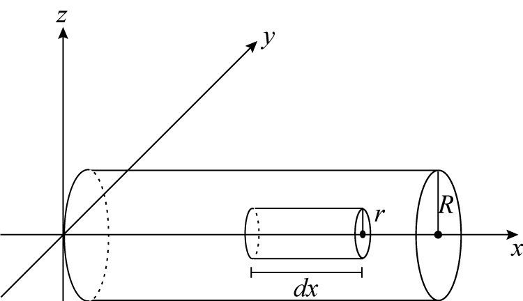
A three dimensional space with two cylinders centered around the x-axis. The larger cylinder has a labeled radius of R. The smaller cylinder has a labled radius of r and a length of $dx$.

Assuming flow in the positive direction, the volume element illustrated in Figure 2 will move because the fluid pressure acting on its left base is greater than that on its right base. On the other hand, a restraining force arising from the fluid's internal friction, or viscosity, is acting in the direction opposite of movement. In general, the force restraining the movement of a layer of fluid by the layer next to it is proportional to their area of contact A and the change of velocity from one layer to the other, divided by the distance over which this change is occurring. In our case,

$F_r=\eta A\cdot {\displaystyle \frac{\mathit{d}v}{\mathit{d}r}}$,

where the constant of proportionality $\eta$ (the Greek letter eta) is called the coefficient of viscosity. In general, the thicker a fluid is, the more viscous it is, with a corresponding higher $\eta$-value. For example, syrup is more viscous than water, motor oil is more viscous than cooking oil, etc.

2. 1. Denoting fluid pressures acting on the two bases of the differential volume element in Figure 2 by P and $P-\mathit{d}P$, respectively, show that the force acting in the positive direction on the volume element is

      $F=\pi r^2\mathit{d}P$.

      (Hint: Remember that $P={\displaystyle \frac{F}{A}}$.)

   2. Show that the restraining force arising from viscosity is

      $F_r=2\pi r\cdot \mathit{d}x\cdot \eta \cdot {\displaystyle \frac{\mathit{d}v}{\mathit{d}r}}$.

   3. Use parts a. and b. to obtain the equation of motion for the volume element. (Hint: Apply Newton's Second Law of Motion, and remember that we are assuming each differential volume element is moving with constant velocity, so its acceleration is zero.)

3. 1. Use the equation of motion you obtained in Question 2c to show that

      $\mathit{d}v={\displaystyle \frac{1}{2\eta }}\cdot {\displaystyle \frac{\mathit{d}P}{\mathit{d}x}}r\mathit{d}r$.

   2. Integrate the above equation to find a formula for $v\left(r\right)$. (Hint: Because the flow is fully developed, ${\displaystyle \frac{\mathit{d}P}{\mathit{d}x}}$ is constant. Don't forget about the constant of integration.)

4. 1. Use the no-slip condition (i.e., the condition $v\left(R\right)=0$) to find the value of the constant of integration in your answer to Question 3b, and verify the formula

      $v\left(r\right)=-{\displaystyle \frac{R^2}{4\eta }}\cdot {\displaystyle \frac{\mathit{d}P}{\mathit{d}x}}\left(1-{\displaystyle \frac{r^2}{R^2}}\right)$.

      (Note that since $v\left(r\right)$ is positive, our formula reflects the fact that ${\displaystyle \frac{\mathit{d}P}{\mathit{d}x}}$ is negative, meaning pressure drops in the direction of flow.)

   2. Given that flow velocity reaches its maximum along the axis (i.e., $v_{\max }=v\left(0\right)$ ), show that

      $v\left(r\right)=v_{\max }\left(1-{\displaystyle \frac{r^2}{R^2}}\right)$.

   3. Conclude that the velocity profile of a fully developed laminar flow is parabolic.

5. Suppose that the centerline speed of a fully developed laminar flow in a circular tube of radius $3\mathrm{cm}$ is $10{\displaystyle \frac{\mathrm{cm}}{\mathrm{s}}}$. Find the equation of the parabola that represents the velocity profile of this flow. (Hint: Place the parabola in the usual xy-system, with its vertex at the origin and opening leftward. Let the vector $v=〈10,0,0〉$ represent a velocity of $10{\displaystyle \frac{\mathrm{cm}}{\mathrm{s}}}$.)

6. If the flow is more turbulent, experiments show that the equation

   $v\left(r\right)=v_{\max }{\left(1-{\displaystyle \frac{r^2}{R^2}}\right)}^{{\displaystyle \frac{1}{p}}}$  ($p>1$)

   better models the fluid velocity within the pipe. For example, $p=7$ provides a fairly accurate model for certain turbulent flows. By choosing appropriate values for r, R, and $v_{\max }$, graph a velocity profile for such a flow. (Answers will vary.)